Accelerate 6G Link-Level Simulation with Batch Processing and GPU Execution

Since R2026a

This example uses:

6G Exploration Library for 5G Toolbox 6G Exploration Library for 5G Toolbox

This example shows how to accelerate pre-6G link-level simulations using batch processing techniques and a graphics processing unit (GPU).

Introduction

In this example you configure a link-level simulation to run on CPU or GPU, with or without batch processing, and profile the impact these options have on runtime.

Batch processing is a way to parallelize simulations with an additional batch dimension to group multiple arrays that would otherwise be processed serially. This example uses a batch dimension to process multiple independent trials of a slot simultaneously, enabling greater statistical coverage. Across the entire transmit-channel-receive processing chain, the bits, grids, symbols, and waveforms use this extra dimension to process more data at once:

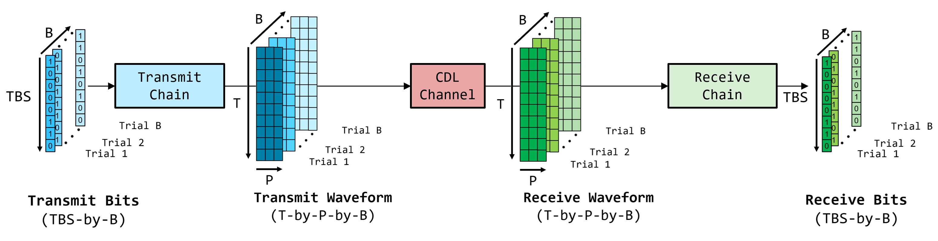
The benefit of using both GPU arrays and a batch dimension together is most noticeable when processing large amounts of data, utilizing more GPU memory at once. The performance benefits you can achieve depend on your specific hardware and code. See Measure and Improve GPU Performance (Parallel Computing Toolbox) and Measure GPU Memory Bandwidth and Processing Power (Parallel Computing Toolbox) for optimization guidance.

This example focuses on the performance benefits of GPU execution with batch processing, which combines multiple iterations into fewer larger array operations within a single worker. This differs from parallel processing with parfor loops, which can distribute independent iterations across multiple CPUs and GPUs, although both approaches can be used together. Refer to the 6G Link-Level Simulation example for extended link-level results, throughput analysis, and more information about different parallelization techniques.

Configure CPU or GPU Execution

GPU execution is enabled in a function when at least one data input argument is a gpuArray object. A gpuArray object is an array stored in GPU memory. The 6G Exploration Library for 5G Toolbox™ supports gpuArray, and functions will execute on GPU automatically when any of the data input arguments to a function are a gpuArray object.

Control whether the simulation runs on CPU or GPU with the UseGPU flag.

Set the UseGPU flag to "on" to run the simulation on GPU, "off" to run on CPU, or "auto" to run on GPU if a compatible GPU device is installed. See GPU Computing Requirements (Parallel Computing Toolbox) for more information.

UseGPU = "off"; % "on", "off" or "auto"

Check that a supported GPU is available and display details of its compute capabilities.

UseGPU = checkGPUAvailability(UseGPU);

Running simulation on CPU.

Set Simulation Parameters

Set the key parameters for the simulation that will impact runtime. You can set further parameters within the setupParameters function.

rng("default");
simParameters = struct();

simParameters.UseGPU = UseGPU;
simParameters.NSizeGrid = 52; % Number of resource blocks
simParameters.NTxAnts = 4;    % Number of transmit antennas
simParameters.NRxAnts = 2;    % Number of receive antennas 
simParameters.NumLayers = 1;  % Number of transmission layers

simParameters = setupParameters(simParameters); % further configuration options

How to Use the Batch Dimension

The batch dimension forms an extra trailing dimension in the arrays passed between functions. This section demonstrates how it works by generating an empty resource grid as an example.

Consider a resource grid where K is the number of subcarriers, L is the number of OFDM symbols, and P is the number of antennas. Now consider the same resource grid with an additional dimension, B, the batch size:

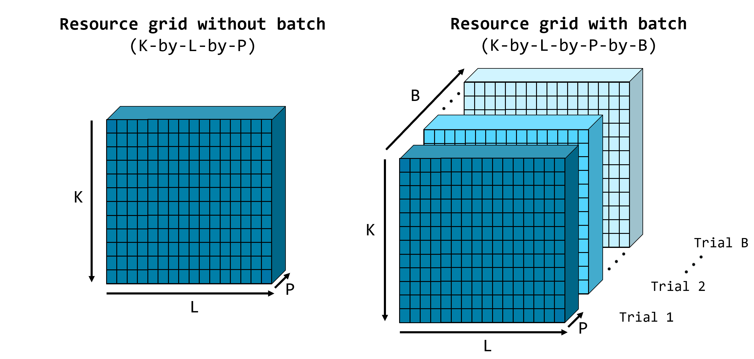
Create a resource grid without a batch dimension:

carrier = pre6GCarrierConfig;
NTxAnts = 4;
txGrid = pre6GResourceGrid(carrier,NTxAnts);
fprintf("K-by-L-by-P Resource grid without batch dimension: [%d %d %d]", size(txGrid,1), size(txGrid,2), size(txGrid,3))

K-by-L-by-P Resource grid without batch dimension: [624 14 4]

Now create the same resource grid with a batch dimension. The BatchSize parameter adds a trailing dimension that groups B independent grids together:

BatchSize = 3;
txGridBatch = pre6GResourceGrid(carrier,NTxAnts,BatchSize=BatchSize);
fprintf("K-by-L-by-P-by-B Resource grid with batch dimension and BatchSize B=3: [%d %d %d %d]", size(txGridBatch,1), size(txGridBatch,2), size(txGridBatch,3), size(txGridBatch,4))

K-by-L-by-P-by-B Resource grid with batch dimension and BatchSize B=3: [624 14 4 3]

Each slice txGridBatch(:,:,:,b) is an independent resource grid for the same slot. Functions across the pre-6G link process B slices simultaneously in a single call, replacing what would otherwise require B iterations of a loop calling each function.

For functions that create data but do not take data inputs, such as pre6GResourceGrid, use the BatchSize name-value argument to control the size of the trailing batch dimension. For functions that process input data, such as pre6GOFDMModulate, output data will automatically have a batch dimension according to the size of the input data.

Configure the Batch Dimension

Simulating multiple independent trials of a simulation helps to improve statistical coverage in results. Set the total number of trials.

simParameters.NumTrials = 100;

In this example, the batch dimension stores multiple trials. This reduces the number of loop iterations required to process each trial by a factor equal to the BatchSize parameter.

The BatchSize defines the size of the trailing dimension of data across function calls. This determines how many transmissions are processed simultaneously. A BatchSize of 1 means that no batch dimension is used.

Set the BatchSize to be a factor of NumTrials.

simParameters.BatchSize = 20; % number of trials stored in batch dimension

Vary the BatchSize to compare the performance benefits of batching. A larger BatchSize moves more work out of the serial loop into vectorized operations, but increases memory usage. Reduce the BatchSize if you encounter maximum variable size limits or GPU out-of-memory errors.

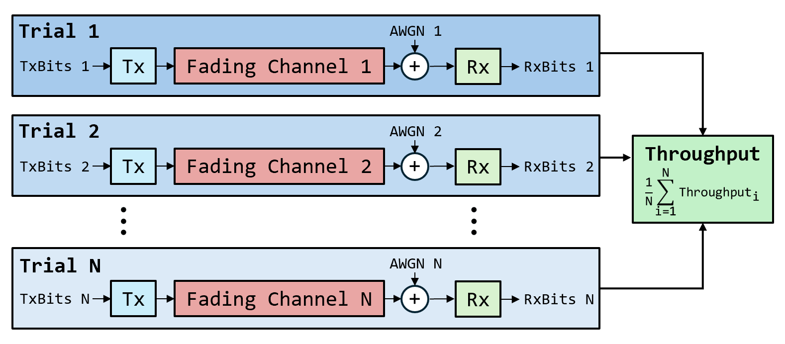
Consider the typical serial processing for running multiple trials of a link, without batch processing. N trials of the same slot-wise simulation are run with different channel realizations (seeds) to improve statistical coverage.

Now consider the same task with batch processing. In this case, each batch dimension is a trial, and B trials constitute a trial batch. Calculate the number of trial batches.

simParameters.NumTrialBatches = ceil(simParameters.NumTrials/simParameters.BatchSize); % number of iterations to process - rounded up when not a factor
fprintf("Simulating %d trial batches (BatchSize = %d).", simParameters.NumTrialBatches, simParameters.BatchSize);

Simulating 5 trial batches (BatchSize = 20).

Using the batch dimension, trials are grouped into trial batches that process multiple trials at once:

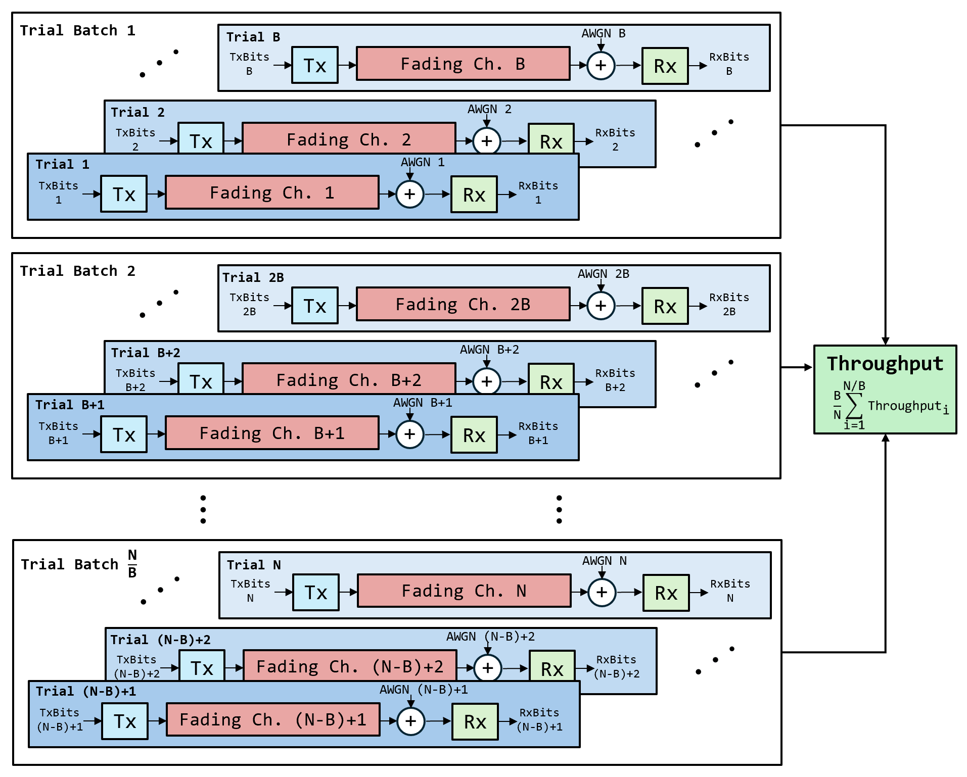
In the batch processing loop, each trial batch has a unique channel seed. To create statistically independent fading channels for each trial in a trial batch, a large time offset (1000 slots) is applied within the same channel seed. The channel fading is deterministic given a seed and time instant, so these widely separated times yield statistically independent realizations. This approach requires that the time offset between batch elements exceeds the channel coherence time, which applies here with 1000-slot separation for a subcarrier spacing of 30 kHz and Doppler shift of 5 Hz. For higher subcarrier spacings with low Doppler shifts, you may need to increase the slot offset to ensure decorrelation.

Construct the link-level simulation to be profiled in the helper function hRunPre6GLink.

function results = runPre6GLink(simParameters)
% Run pre-6G link simulation across trial batches

    % Channel seeds for each trial batch
    chSeed = randi([0 2^32-1],[1 simParameters.NumTrialBatches]); 

    % Pre-allocate results
    numCodedBits = 0;
    numCodedBitErrors = 0;
    blkErrors = 0;
    numTrBlks = 0;

    % Trial batches loop
    for it = 1:simParameters.NumTrialBatches
    
        results = hRunPre6GLink(simParameters, simParameters.snr, chSeed(it));
    
        numCodedBits = numCodedBits + results.NumCodedBits;
        numCodedBitErrors = numCodedBitErrors + results.NumCodedBitErrors;
        blkErrors = blkErrors + results.NumBlkErrors;
        numTrBlks = numTrBlks + results.NumTrBlks;
    
    end

    % Results
    BER = double(numCodedBitErrors) / double(numCodedBits);
    BLER = double(blkErrors) / double(numTrBlks);
    results.BER = BER;
    results.BLER = BLER;

end

The focus of this example is runtime performance. For analysis of throughput performance, see the 6G Link-Level Simulation example.

Profile Simulation

Run and profile the pre-6G link simulation contained within the runPre6GLink function.

The profiling code is contained within the profileLink function (see Local Functions). This uses the gputimeit function to measure the typical time in seconds it takes to run the function with GPU execution enabled. For CPU execution, this function uses timeit instead. The total runtime displayed is the average time taken to execute the runPre6GLink function, after simulation set-up and configuration above.

[runTime,execDevice,results] = profileLink(simParameters);
fprintf("Total simulation runtime with %s execution and batch size of %d is: %.2f seconds",execDevice,simParameters.BatchSize,runTime)

Total simulation runtime with CPU execution and batch size of 20 is: 6.85 seconds

Compare this runtime against the same simulation run on CPU with a BatchSize of 1 to examine the speed-up achieved.

refB = simParameters.BatchSize;
simParameters.UseGPU = "off";
simParameters.BatchSize = 1;
simParameters.NumTrialBatches = ceil(simParameters.NumTrials/simParameters.BatchSize); % update number of trial batches
runTimeRef = profileLink(simParameters);
if execDevice == "GPU"
    fprintf("Speed-up factor of %.2f using GPU execution with a batch size of %d compared to CPU execution and batch size of 1.",runTimeRef/runTime,refB)
else
fprintf("Speed-up factor of %.2f using CPU execution with a batch size of %d compared to a batch size of 1.",runTimeRef/runTime,refB)
end

Speed-up factor of 2.16 using CPU execution with a batch size of 20 compared to a batch size of 1.

Extended Performance Analysis

Effect of Batch Size on Runtime

Run the section below to examine the impact of varying the BatchSize on total simulation runtime. This profiles the simulation for 100 trials across a range of batch sizes from 1 to 100 and plots the runtime trend.

runBatchComparison = false;

if runBatchComparison

    simParameters.NumTrials = 100; 
    B = [1 2 5 10 25 50 100];
    
    runTimes = zeros(numel(B),1);

    for i = 1:numel(B)

        simParameters.BatchSize = B(i);
        simParameters.NumTrialBatches = ceil(simParameters.NumTrials/simParameters.BatchSize); % update number of trial batches
        runTimes(i) = profileLink(simParameters);

    end

    figure;
    plot(B,runTimes,"-*")
    title("Runtime vs. Batch Size")
    xlabel("Batch Size");
    ylabel("Runtime [s]");
    grid on

end

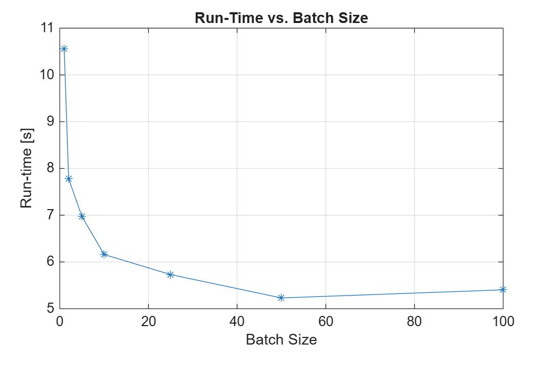
(Reference graphic generated on NVIDIA RTX 6000 Ada Generation GPU)

While batch processing accelerates runtime, there is a limit to the achievable performance benefit that comes with increasing the BatchSize for a given amount of work.

Reference Results

The following table details reference runtime results for extended simulation configurations of this example, varying the grid size and number of antennas:

Execution	`BatchSize`	`NumTrials = 100` `NSizeGrid = 52` `NTxAnts = 4` `NRxAnts = 2`	`NumTrials = 100` `NSizeGrid = 104` `NTxAnts = 8` `NRxAnts = 2`
CPU	1	10.66 s	14.50 s
CPU	100	5.22 s	7.80 s
GPU	1	13.32 s	15.74 s
GPU	100	2.03 s (5.3x faster than CPU, B=1)	3.41 s (4.3x faster than CPU, B=1)

GPU results were generated with an NVIDIA RTX 6000 Ada Generation GPU.

This shows that GPU execution with batch processing offers up to a 5.3x speed-up compared to CPU execution without batch processing. With CPU execution alone, batch processing offers up to a 2x speed-up.

Local Functions

function [runTime,execDevice,results] = profileLink(simParameters)
% Profile the link-level simulation for CPU or GPU execution

    f = @() runPre6GLink(simParameters); % create function handle required by gputimeit and timeit

    if simParameters.UseGPU == "on" || simParameters.UseGPU == "auto" && canUseGPU
        execDevice = "GPU";
        runTime = gputimeit(f);
    else
        execDevice = "CPU";
        runTime = timeit(f);
    end

    results = runPre6GLink(simParameters); % BER and BLER

end

function simParameters = setupParameters(simParameters)
% Setup additional simulation parameters

    simParameters.SubcarrierSpacing = 30; % kHz
    mcsTables = nrPDSCHMCSTables();
    simParameters.MCSTable = mcsTables.QAM64Table; % MCS table
    simParameters.MCS = 18; % MCS
    simParameters.PRGBundleSize = 4; % PRB bundling: any positive power of 2, or [] to signify "wideband"
    
    simParameters.DelayProfile = "CDL-C";
    simParameters.DelaySpread = 300e-9;
    simParameters.MaximumDopplerShift = 5;
    simParameters.PerfectChannelEstimator = false;

    simParameters.NHARQProcesses = 1;
    simParameters.EnableHARQ = false;
    simParameters.rvSeq = [0 2 3 1];

    simParameters.snr = 0; % SNR point

    simParameters.NumSlotsPerTrial = 1; % Number of slots (sequential slot positions)

end

function UseGPU = checkGPUAvailability(UseGPU)
% Check GPU availability and display device details

    if UseGPU == "on" || UseGPU == "auto"
        if canUseGPU
            fprintf("Running simulation on GPU. \n");
            fprintf("GPU Details: %s device, %d multiprocessors, %s compute capability.\n", ...
                gpuDevice().Name, gpuDevice().MultiprocessorCount, gpuDevice().ComputeCapability);
        else
            warning("No supported GPU is available - running simulation on CPU.");
            UseGPU = "off";
        end
    else
        fprintf("Running simulation on CPU.");
    end

end