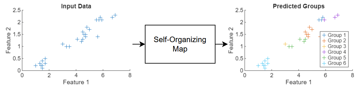
Cluster Data Using Self-Organizing Map (SOM)

Since R2026a

This example shows how to train a self-organizing map (SOM) neural network to cluster unlabeled data.

Data clustering is the task of grouping similar observations in a dataset. Typically, clustering is an unsupervised learning task. You do not need a labeled set of training data to train the model. The model does not assign semantic labels to the inputs. The model is trained to output the same group index for similar observations.

A self-organizing map is a type of neural network that performs clustering. It maps high-dimensional data to positions in a lower-dimensional space. The learnable parameters are weight vectors that represent reference points in the space of the training data. During training, the network updates these weight vectors so that similar inputs map to nearby locations in the lower-dimensional space. This process preserves the topological relationships of the original data.

This diagram shows the flow of data through a SOM neural network.

This example trains a SOM neural network that clusters flowers using measurements that correspond to petal and sepal length and width.

Load Training Data

Load the Iris example dataset from iris_dataset. This dataset contains measurements of 150 flowers. The measurements are sepal length, sepal width, petal length, and petal width. Transpose the data so that

load iris_dataset
X = irisInputs';

Visualize the data in a plot matrix. The plot in row $$i$$ column $$j$$ is a scatter plot of feature $$i$$ and feature $$j$$. The histograms on the diagonal show the distribution of the corresponding feature values.

figure
plotmatrix(X)
title("Data Features")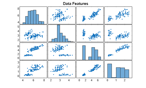

Split the data into training, validation, and test partitions using the trainingPartitions function, which is attached to this example as a supporting file. To access this function, open the example as a live script. Use 80% of the data for training and the remaining 20% for testing.

numObservations = size(X,1);
[idxTrain, idxTest] = trainingPartitions(numObservations,[0.8 0.2]);
XTrain = X(idxTrain,:);
XTest = X(idxTest,:);

Define Neural Network Architecture

Define the neural network architecture for the SOM.

• Use a feature input layer with an input size that matches the number of features.

• For the SOM operation, use the custom layer somLayer, attached to this example as a supporting file. to access this layer, open the example as a live script. Use a 3-by-2 grid. To initialize the weights, specify the training data.

gridSize = [3 2];

numFeatures = size(XTrain,2);

layers = [
    featureInputLayer(numFeatures)
    somLayer(gridSize,XTrain)];

Define Model Function

To train the SOM neural network, create a model function that takes the training data as input and returns the normalized neighborhood-augmented activations and the indices of any inactive groups in the map.

The normalized neighborhood-augmented activations represent how strongly the SOM weights respond to the input. They take into account both the closest weight vector and its neighboring nodes. The model uses them to simulate cooperative learning during training, and ensures that similar inputs have similar activations and preserve topological relationships in the map.

function [Y, idxInactive] = model(net,X,iteration,initialNeighborhoodRadius, ...
    numOrderingIterations,somLayerName)

arguments
    net
    X
    iteration
    initialNeighborhoodRadius
    numOrderingIterations
    somLayerName = "som"
end

% Make predictions.
Y = predict(net,X);

% Add noise.
mask = rand(size(Y)) < 0.9;
Y = Y.*mask;

% Calculate new radius.
r = initialNeighborhoodRadius;
N = numOrderingIterations;
rNew = 1 + (r-1)*(1 - (iteration - 1)/N);

% Determine neighborhood.
layer = getLayer(net,somLayerName);
distances = layer.NodeDistances;
neighborhood = distances <= rNew;

% Augment activations and normalize.
Y = Y*neighborhood + Y;
sumY = sum(Y,1);
Y = Y./sumY;

% Find inactive nodes.
idxInactive = sumY == 0;

end

Specify Training Options

Specify the training options. Choosing among the options requires empirical analysis. To explore different training option configurations by running experiments, you can use the Experiment Manager app.

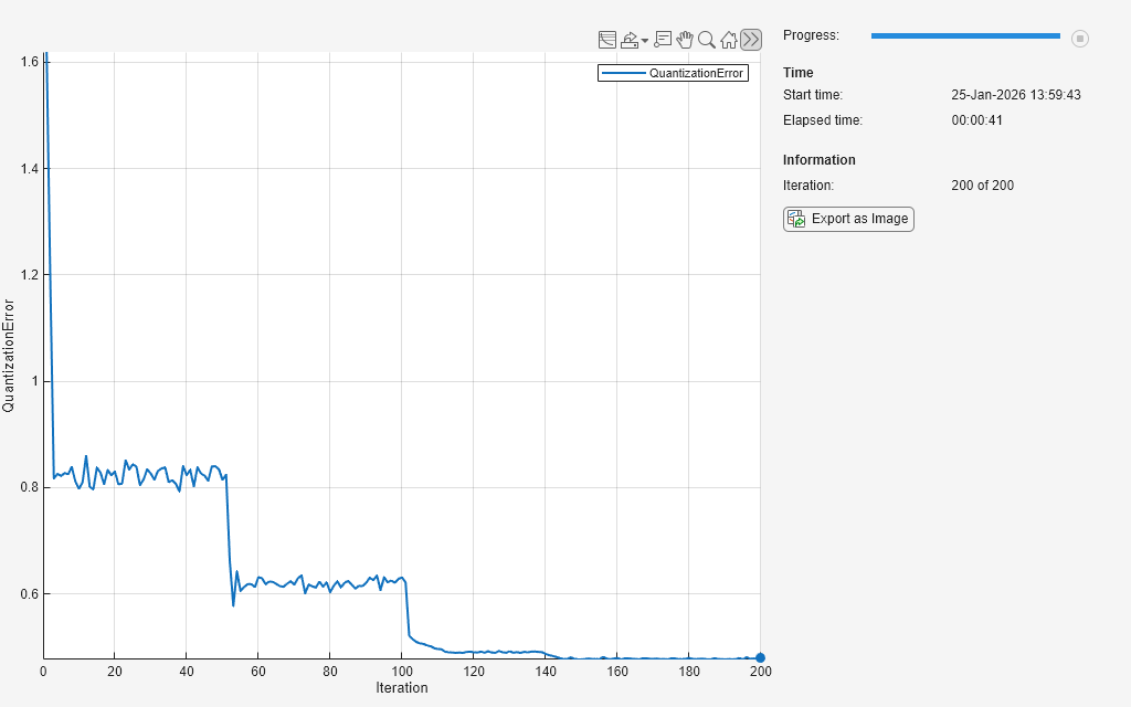
• Train the network for 200 iterations.

• Train with 100 ordering iterations.

• Use an initial neighborhood with a radius size of three.

numIterations = 200;
numOrderingIterations = 100;
initialNeighborhoodRadius = 3;

Define SOM Update Function

Define a custom update function that updates the SOM weights using the model activations and the indices of the inactive groups.

function net = somupdate(net,X,Y,idxInactive,somLayerName)

arguments
    net
    X
    Y
    idxInactive
    somLayerName = "som"
end

% Extract weights.
idxSom = net.Learnables.Layer == somLayerName;
idxWeights = net.Learnables.Parameter == "Weights";
idx = idxSom && idxWeights;
weights = net.Learnables.Value{idx};

% Calculate new weights.
newWeights = X'*Y;
dWeights = newWeights - weights;
dWeights(:,idxInactive) = 0;
newWeights = weights + dWeights;

% Update learnables.
net.Learnables.Value{idx} = dlarray(newWeights);

end

Train Neural Network

Train the neural network using a custom training loop.

To make predictions with the neural network, convert the layer array to a dlnetwork object.

net = dlnetwork(layers);

Initialize the training progress monitor.

monitor = trainingProgressMonitor( ...
    Metrics="QuantizationError", ...
    Info="Iteration", ...
    XLabel="Iteration");

Train the neural network. For each iteration:

• Calculate the model activations and the indices of the inactive groups using the model function.

• Update the learnable parameters using the custom somupdate function.

• Update the training progress monitor using the quantizationError function, listed in the Quantization Error Function section of the example.

iteration = 0;

while iteration < numIterations && ~monitor.Stop
    iteration = iteration + 1;
    [Y, idxInactive] = model(net,XTrain,iteration, ...
        initialNeighborhoodRadius,numOrderingIterations);

    net = somupdate(net,XTrain,Y,idxInactive);

    layer = getLayer(net,"som");
    weights = layer.Weights;
    qe = quantizationError(weights,XTrain);

    recordMetrics(monitor,iteration,QuantizationError=qe);
    
    updateInfo(monitor, ...
        Iteration=iteration + " of " + numIterations);

    monitor.Progress = 100*iteration/numIterations;
end

Test Neural Network

Because clustering is an unsupervised learning task, there are no labels to help evaluate the accuracy of the neural network. Instead, you must evaluate the test predictions manually.

Make predictions with the neural network. To convert the network outputs to integer values, use the onehotdecode function and specify the output class type as "double".

numGroups = prod(gridSize);
groupNames = "Group " + string(1:numGroups);
Y = minibatchpredict(net,XTest);
Y = onehotdecode(Y,groupNames,2);

Calculate the quantization error.

layer = getLayer(net,"som");
weights = layer.Weights;
qeTest = quantizationError(weights,XTest)

qeTest = 
0.5543

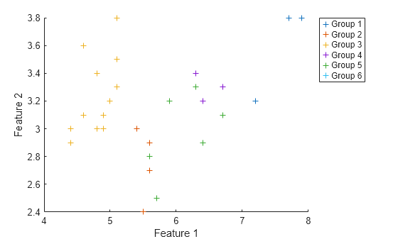
Visualize the predicted groups against the first two features in a scatter plot.

figure
hold on
for i = 1:numGroups
    idx = double(Y) == i;
    scatter(XTest(idx,1),XTest(idx,2),"+");
end
xlabel("Feature 1")
ylabel("Feature 2")
legend(groupNames,Location="bestoutside")

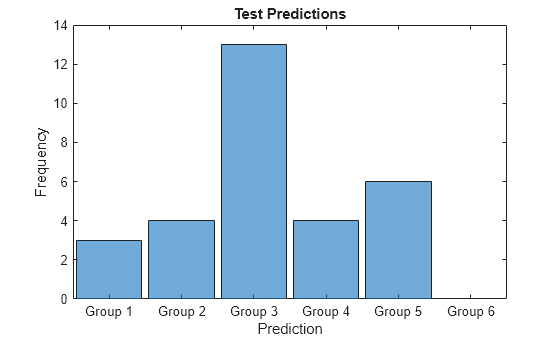
Visualize the distribution of the predicted groups in a histogram.

figure
histogram(Y)
xlabel("Prediction")
ylabel("Frequency")
title("Test Predictions")

Visualize the SOM hits in a heatmap. Using the predictions, extract the corresponding group positions from the SOM layer. For each of the nodes in the SOM grid, display the count of the corresponding prediction.

YPositions = layer.Positions(:,Y);
M = histcounts2(YPositions(1,:),YPositions(2,:));

figure
heatmap(M)
title("SOM Hits")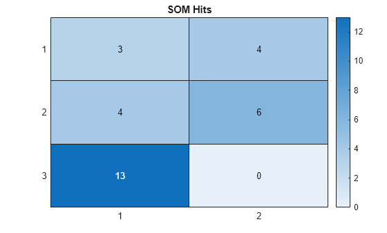

Quantization Error Function

In the context of self-organizing maps, the quantization error measures how well the SOM weights represent the input data.

The quantizationError function takes the SOM weights and the network input data as input and returns the mean of the euclidean distances between each input vector and the closest weight vector. A lower quantization error indicates a closer match between the SOM representation and the input data.

function qe = quantizationError(weights,X)
    numObservations = size(X,1);
    minDistances = zeros(numObservations,1);

    for i = 1:numObservations
        diffs = weights' - X(i,:);
        distances = sqrt(sum(diffs.^2,2));
        minDistances(i) = min(distances);
    end

    qe = mean(minDistances);
end

Copyright 2025 The MathWorks, Inc.