Configure Experiment to Solve Ordinary Differential Equations Using Template

Since R2024b

Experiment Manager provides templates to streamline experiment setup. Rather than starting with a blank experiment, you can use a template to save time. This example shows how to use the Solve System of Ordinary Differential Equations template as a starting point for solving a system of two first-order ODEs.

$\begin{array}{l}{x_1}^{\prime }=x_2\\ {x_2}^{\prime }=\mu \left(1-{x_1}^2\right)x_2-x_1\end{array}$

Create Experiment Using Template

You can access templates on the Experiment Manager start page. Open the Experiment Manager app. Then, on the start page, click New > Project > Blank Project, and choose the Solve System of Ordinary Differential Equations template.

This template automatically generates an experiment that includes a sample initialization function, a set of default parameters, and an experiment function designed for solving ODEs.

Specify Initial Conditions

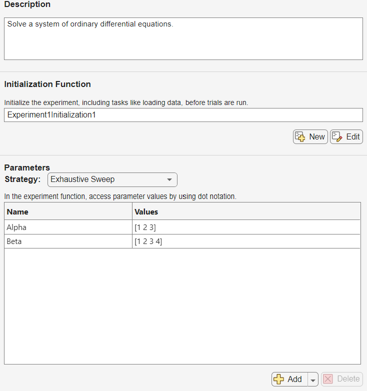
To specify the initial conditions for your system, modify the initialization function. When you run an experiment, Experiment Manager executes the initialization function once before beginning the experiment trials. To open the initialization function file in the MATLAB Editor, click Edit in the Initialization Function section.

For example, to solve a system where the initial value of $x_1$ is 2 and the initial value of $x_2$ is 0, specify the output of the initialization function as [2 0].

function output = Experiment1Initialization1()
output = [2 0];
end

Then save and close your initialization function file.

Customize Parameters

The Solve System of Ordinary Differential Equations template includes two parameters, Alpha and Beta, which you can customize for your experiment. If you want to specify the end time for the experiment as an additional parameter, you can click Add > Add From Suggested List, select the endTime parameter, and specify a vector of values. Alternatively, you can set a scalar end time directly within the experiment function.

For example, replace the name of parameter Alpha with Mu, and assign the parameter a range of values from 1 to 5. Because this example does not require a second parameter, select the second row in the table of parameters and click Delete.

Name	Values
Mu	1:5

Customize Functions to Solve

After you specify the initial conditions and parameters, modify the experiment function to represent your system. To open the experiment function, click Edit in the Experiment Function section of the experiment editor. The experiment function for this template also creates a plot for each trial to visualize the values of $x_1$ and $x_2$ over time.

In the function code, you can access the initial values using params.InitializationFunctionOutput. For example, compute the solution of the van der Pol equation over the time range [0 15] using the ode45 function. Modify the plotting code by changing the title to include the value of parameter Mu for the plotted trial.

function [x1max,x2max] = Experiment1Function1(params)
xInitial = params.InitializationFunctionOutput;
Mu = params.Mu;

if ~isfield(params,"endTime")
    params.endTime = 15;
end
tRange = [0 params.endTime];

function dxdt = odefun(t,x)
    dxdt = [x(2); Mu*(1-x(1)^2)*x(2)-x(1)];
end
[t,x] = ode45(@odefun,tRange,xInitial);

figure(Name="x1 and x2 over Time")
plot(t,x,"-o")
title(["Solutions When Mu = " + num2str(Mu)])
xlabel("Time")
ylabel("Value")
legend("x1","x2")

x1max = max(x(:,1));
x2max = max(x(:,2));
end

Then save and close your experiment function file.

Run Experiment and View Results

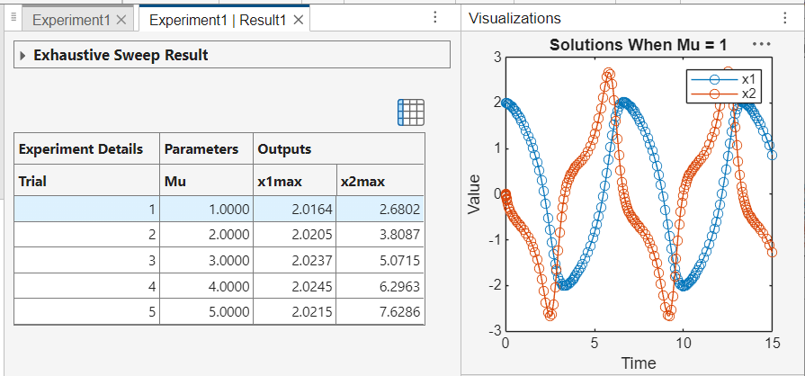
To run your experiment, click Run on the Experiment Manager toolstrip. For this example, the app runs the experiment function for each value of parameter Mu and displays the results in a table.

To display the plot that the experiment function created for a trial, select a trial in the results table and then click the plot in the Review Results section of the toolstrip. You can use these plots to quickly assess how different parameter values affect the system.

To further analyze the experiment results, you might want to refine the parameter range or decrease the step size and rerun the experiment.

You can also export the results table to the MATLAB workspace and perform computations using the results. To export the results, click Export > Export All Trials on the toolstrip.