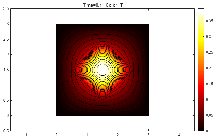
Heat Transfer Between Two Squares Made of Different Materials: PDE Modeler App

Solve the following heat transfer problem with different material parameters. This example uses the PDE Modeler app. For the command-line solutions see Heat Transfer Between Two Squares Made of Different Materials.

The 2-D geometry for this problem is a square with an embedded diamond (a square with 45 degrees rotation). PDE governing this problem is a parabolic heat equation:

$$\rho C\frac{\partial T}{\partial t}-\nabla \cdot \left(k\nabla T\right)=Q+h\left(T_{\text{ext}}-T\right)$$

where ρ is the density, C is the heat capacity, k is the coefficient of heat conduction, Q is the heat source, h is convective heat transfer coefficient, and T_ext is the external temperature.

To solve this problem in the PDE Modeler app, follow these steps:

1. Model the geometry: draw the square region with corners in (0,0), (3,0), (3,3), and (0,3) and the diamond-shaped region with corners in (1.5,0.5), (2.5,1.5), (1.5,2.5), and (0.5,1.5).

   pderect([0 3 0 3])
   pdepoly([1.5 2.5 1.5 0.5],[0.5 1.5 2.5 1.5])

2. Set the x-axis limit to [-1.5 4.5] and y-axis limit to [-0.5 3.5]. To do this, select Options > Axes Limits and set the corresponding ranges.

3. Set the application mode to Heat Transfer.

4. The temperature is kept at 0 on all the outer boundaries, so you do not have to change the default Dirichlet boundary condition T = 0.

5. Specify the coefficients. To do this, select PDE > PDE Mode. Then click each region and select PDE > PDE Specification or click the button on the toolbar. Since you are solving the parabolic heat equation, select the Parabolic type of PDE for both regions. For the square region, specify the following coefficients:

   • Density, pho = 2

   • Heat capacity, C = 0.1

   • Coefficient of heat conduction, k = 10

   • Heat source, Q = 0

   • Convective heat transfer coefficient, h = 0

   • External temperature, Text = 0

   For the diamond-shaped region, specify the following coefficients:

   • Density, pho = 1

   • Heat capacity, C = 0.1

   • Coefficient of heat conduction, k = 2

   • Heat source, Q = 4

   • Convective heat transfer coefficient, h = 0

   • External temperature, Text = 0

6. Initialize the mesh by selecting Mesh > Initialize Mesh. For a more accurate solution, refine the mesh by selecting Mesh > Refine Mesh.

7. Set the initial value and the solution time. To do this, select Solve > Parameters.

   The dynamics for this problem is very fast — the temperature reaches steady state in about 0.1 time units. To capture the interesting part of the dynamics, set time to logspace(-2,-1,10). This gives 10 logarithmically spaced numbers between 0.01 and 0.1. Set the initial value of the temperature u(t₀) to 0.

8. Solve the equation by selecting Solve > Solve PDE or clicking the button on the toolbar.

9. Plot the solution. By default, the app plots the temperature distribution at the last time. The best way to visualize the dynamic behavior of the temperature is to animate the solution. To do this, select Plot > Parameters and select the Animation and Height (3-D plot) options to animate a 3-D plot. Also, you can select the Plot in x-y grid option to use a rectangular grid instead of the default triangular grid. Using a rectangular grid instead of a triangular grid speeds up the animation process significantly.

   You can also plot isothermal lines using a contour plot and the heat flux vector field using arrows.

   1. Select Plot > Parameters.

   2. In the resulting dialog box, deselect the Animation, and Height (3-D plot), and Plot in x-y grid options.

   3. Change the colormap to hot by using the corresponding drop-down menu in the same dialog box.

   4. To obtain the first plot, select the Color and Contour options.

   5. For the second plot, select the Color and Arrows and set their values to temperature and heat flux, respectively.

   Isothermal Lines

   

   Temperature and Heat Flux