Examine Approaches to Fine Tune a Deployed Policy

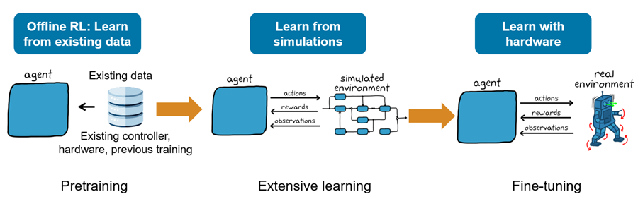
While learning a policy by interacting with a simulated environment has many practical advantages, there can be a substantial "reality gap" between the simulated environment and real word conditions. This gap often results from factors such as inaccurate or unknown model dynamics and environmental conditions. For these reasons, it might be necessary to refine a deployed policy using data collected from in real world conditions, to ensure it can effectively and safely solve a real-world task.

If data collected from previous simulation, (or real world data), is available, offline reinforcement learning can be used to pre-train the agent. The pretrained agent can then be further improved by interacting with a simulated environment. Finally, to refine the policy so it can also learn in real world conditions, you can deploy it on control hardware. This picture illustrates the workflow.

When deploying an agent to the real world, in theory, you could use a few different architectures to allocate the required computations.

Agent Runs on Desktop and Interacts with Real World

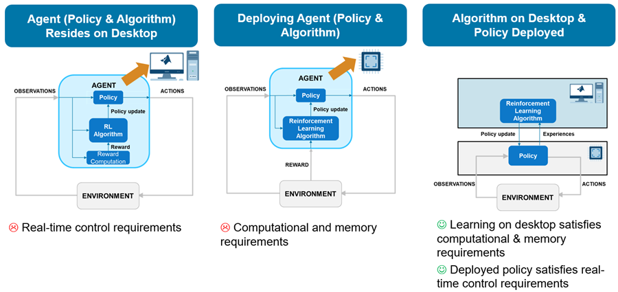
The first (simplest) architecture would rely on a custom MATLAB environment that sends actions and receives observations from the physical system. The agent then interacts with the custom environment within a reinforcement learning loop running in a MATLAB desktop process. In this architecture, the hardware applies the received actions to the physical system, then measures new observations and sends them back to the MATLAB desktop process.

The problem with this first approach is that the time that the agent needs to learn and execute its policy is both unpredictable, because the MATLAB process typically runs within a non-realtime operating system, and often longer than the sampling time needed to safely and successfully control the physical system. For similar reasons, the time needed to send actions and receive observations over a communication channel is also unpredictable and has a latency that is hard to constrain. So, this first architecture typically cannot accommodate for the real time and sampling rate constraints needed to control the physical system unless the physical system dynamics are sufficiently slow.

Agent Runs on Dedicated Hardware Board

A second possible way to allocate the required computations is to generate lower level code (typically C/C++) for the agent and deploy the generated code on a dedicated hardware board that interacts with the physical system. This board typically runs a real time operating system, or at least an operating system with predictable process latency.

The problem with this second approach is that a typical dedicated controller board lacks the memory and computational power necessary to run the agent learning algorithm, especially for off-policy agents. In other words, this second approach might be feasible only by using a very powerful on-board computer with an appropriately capable data acquisition board.

Desktop Algorithm Trains Deployed Policy

A third possible architecture separates the control policy from the learning algorithm. Specifically, the control policy runs on a dedicated experiment process (typically on a controller board) while the learning algorithm runs in a MATLAB process on a desktop computer. Here, differently from the previous architectures, learning happens asynchronously with respect to the hardware process, that is, the policy process computes actions independently of any learning that might take place.

This architecture makes it easier to satisfy real-time constraints, especially on systems with fast sample times, since the experiment process is not directly concerned with learning. Furthermore, the learning process can be executed on a powerful machine with a powerful GPU to accelerate learning.

In this architecture, the experiment process collects experiences by interacting with the physical system and periodically sends these experiences to the learning process. The learning process then uses the experiences received from the policy process to update the learnable parameters of the agent, and then periodically sends the updated parameters to the experiment process. The experiment process then updates its policy parameters with the new parameters received by the learning process. For an example implementing this architecture, see Train Policy Deployed on Raspberry Pi.

Summary: Advantages and Disadvantages

This picture illustrates the advantages and disadvantages of the three architectures.

Transferring a policy that has been trained in a simulated environment to a real-world setting is also referred to as a "Sim to Real" workflow. There are several intermediate verification steps that can facilitate such workflow, such as Software In the Loop (SIL, in which the code generated from the agent or policy runs in within a simulation), Processor In the Loop (PIL, in which the generated code from the agent or policy runs on a dedicated board and interacts with the simulation) and Hardware In the Loop (HIL, in which a model of the environment runs in real time on dedicated hardware). For an example showing how you can apply the SIL and PIL steps to a policy (that does not need to learn after deployment), see Run SIL and PIL Verification for Reinforcement Learning. For more information, see SIL and PIL Simulations (Embedded Coder).