Running AMI Models in MATLAB

Since R2025a

This example shows how to run statistical and time domain signal integrity simulations using IBIS-AMI models in MATLAB®. This workflow mimics the workflow of an EDA tool such as Signal Integrity Toolbox's apps Serial Link Designer and Parallel Link Designer. The main advantage of this workflow is the full control of all aspects of the simulation, but this can also be a disadvantage as the complexity is high.

The Tx and Rx IBIS-AMI models are attached with the example. A MATLAB script runAMI is also attached with the example. The runAMI script contains the the same code flow and you can run it without going through the example steps.

Simulation Setup

Set up the base simulation parameters such as symbol time, number of samples per bit, sample interval, modulation scheme, target BER, simulation UI, and ignore UI. You can adjust the number of UI simulated and UI ignored to vary the length of the time domain simulation.

%% Simulation setup
symbolTime = 100e-12;
samplesPerBit = 16;
sampleInterval = symbolTime/samplesPerBit;
modulation = 3;
targetBER = 1e-6;
numSimulationUI = 20000;
ignoreUI = 10000;

Stimulus Setup

The statistical simulation is impulse response based. So you only need to set up the stimulus for the time-domain simulation. Use the serdes.Stimulus System object™ to generate that pattern. Note that blockSize, which is the size of the block of samples that is passed to the time domain (GetWave) portion of the IBIS-AMI models, is variable here. Typically, in an EDA tool, blockSize is set to a proportionally small number such as 1024 to keep the memory requirements of simulations lean. GetWave is called multiple times in a loop with a smaller blockSize chunks until the total waveform is fully processed. Using a low block size is not a requirement and for simplicity in this example, GetWave is called only once with the entire length of the time domain stimulus.

%% Stimulus setup
stimulus = serdes.Stimulus;
stimulus.SymbolTime = symbolTime;
stimulus.SampleInterval = sampleInterval;
stimulus.Modulation = modulation;
stimulusSamples = numSimulationUI*samplesPerBit;
stimulusWave = zeros(stimulusSamples,1);
for stimulusWaveIdx = 1:stimulusSamples
    stimulusWave(stimulusWaveIdx) = stimulus();
end
blockSize = stimulusSamples;

Channel Setup

This examples uses the serdes.ChannelLoss System object to generate the channel to serve both the statistical and time-domain portions of the simulation. The channel used in this example is a lossy one and is configured with a target frequency at the fundamental frequency of the simulation. The example also includes a simple Tx and Rx analog model. Note that the IBIS file attached to the example is not used for the analog models directly although it was generated with the same parameters as shown. If you want to use a more advanced analog model from an externally generated IBIS model, use the Serial Link Designer or Parallel Link Designer app to create an impulse response and substitute the existing response. For the simulation, the impulse response is used directly in the statistical portion where the channel object is used to apply the channel to the time domain waveform. Similar to the blocksize parameter from the Stimulus section, rowSize represents the length of the impulse response representing the channel.

%% Channel setup
channel = serdes.ChannelLoss;
% Lossy channel
channel.dt = sampleInterval;
channel.TargetFrequency = 1/symbolTime/2;
channel.Loss = 16; %dB
channel.Zc = 100;
% Tx analog model
channel.TxR = 50;
channel.TxC = 100e-15;
channel.RiseTime = 10e-12;
channel.VoltageSwingIdeal = 1;
% Rx analog model
channel.RxR = 50;
channel.RxC = 200e-15;
% Access impulse
channelImpulse = channel.impulse;
rowSize = size(channelImpulse,1);

AMI Model Setup

The SerDes Toolbox AMI system object serves as the core of the simulation described in this example. You will create two instances, one for the Tx and one for the Rx. Each is configured with important simulation, stimulus, and channel parameters previously determined in the example. Two files are associated with running each IBIS-AMI algorithmic model. The first file is the library executable, where LibraryPath is configured with the path to the directory containing it and then the LibraryName is the name without the file extension. This flow supports both Windows and Linux OS, so the library will with have a dll or so extension (both are included with the example). The other primary file is the ami file that contains all the IBIS-AMI parameters that control the model. This file has a specific format outlined extensively in the IBIS-AMI standard with each line describing a parameter and its valid settings. Feed this control information into an IBIS-AMI model using an input string, again with a specific format. The serdes.AMI system object has a convenience function that takes an AMI input and generates an input string with default parameter value. This input string can then be carefully edited if necessary, making sure to stay within the constraints provided in the file. For this example, all default parameter values were used.

disp(serdes.AMI.generateDefaultInputString('serdes_tx.ami'));

(serdes_tx(Modulation_Levels 3)(FFE(Mode 1)(TapWeights(-1 0)(0 1)(1 0)(2 0))))

disp(serdes.AMI.generateDefaultInputString('serdes_rx.ami'));

(serdes_rx(Modulation_Levels 3)(CTLE(Mode 2)(ConfigSelect 0)(SliceSelect 0))(DFECDR(ReferenceOffset 0)(PhaseOffset 0)(Mode 2)(TapWeights(1 0)(2 0)(3 0)(4 0)(5 0)(6 0)(7 0)(8 0))))

Based on the input strings, it can be seen that the Tx contains a FFE and the Rx a CTLE and DFECDR. The input strings are generated inline below.

%% Tx and Rx AMI setup
% Tx
txAMI = serdes.AMI;
txAMI.LibraryPath = pwd;
txAMI.LibraryName = ['serdes_tx_' computer('arch')];
txInputString = txAMI.generateDefaultInputString('serdes_tx.ami');
txAMI.InputString = txInputString;
txAMI.InitOnly = false;
txAMI.SkipFirstBlock = false;
txAMI.SymbolTime = symbolTime;
txAMI.SampleInterval = sampleInterval;
txAMI.RowSize = rowSize;
txAMI.BlockSize = blockSize;
% Rx
rxAMI = serdes.AMI;
rxAMI.LibraryPath = pwd;
rxAMI.LibraryName = ['serdes_rx_' computer('arch')];
rxInputString = rxAMI.generateDefaultInputString('serdes_rx.ami');
rxAMI.InputString = rxInputString;
rxAMI.InitOnly = false;
rxAMI.SkipFirstBlock = false;
rxAMI.SymbolTime = symbolTime;
rxAMI.SampleInterval = sampleInterval;
rxAMI.RowSize = rowSize;
rxAMI.BlockSize = blockSize;

Simulation

Modify the channel impulse response and the stimulus waveform using the Tx AMI object. You need to pass the stimulus through the channel to generate only the time-domain waveform. Then call the Rx AMI object with the channel waveform output and the modified impulse from the Tx. When you close out the simulation, release both AMI objects to free up memory and flush the simulation metadata to the AMIData parameter structures in each object. Note that a ClockIn parameter set to -1is provided to each AMI object. This parameter is used for clock forwarding IBIS-AMI models, which is only supported in the Simulink® AMI block.

%% Simulation
ClockIn = -1;
[txWaveOut, txImpulseOut] = txAMI(stimulusWave, channelImpulse, ClockIn);
channelWaveOut = channel(txWaveOut);
[rxWaveOut, rxImpulseOut] = rxAMI(channelWaveOut, txImpulseOut, ClockIn);

%% Cleanup and flush results
txAMI.release;
rxAMI.release;

Processing Results

Now that the simulation is complete, the resulting impulse and waveform data can be processed and visualized. Some of the data must be pre-processed prior to using in the analysis. For statistical analysis, the impulse is converted to a pulse response. For time domain analysis, ignore UI must be removed from the leading edge of the waveform and Rx clock times which are in the AMIData struct. Both analysis' need threshold information output from the Rx AMI in the output string (similar to the input string). This is also part of the AMIData meta data struct that is accessed in the object. A helper function is provided to parse out the thresholds from the other parameters in the output string. The results processing and visualization is also done in helper functions using various SerDes Toolbox and Signal Integrity Toolbox utilities. For this example, the statistical and time domain eyes are plotted in addition to the eye height of the PAM3 eyes. Many other metrics are part of the metric structures that are created.

The results processing and visualization is done in helper functions using various SerDes Toolbox and Signal Integrity Toolbox utilities. For this example, the statistical and time domain eyes are plotted in addition to the eye height of the PAM3 eyes. Many other metrics are available as part of the metric structures that are created.

Before you perform any analysis, some of the simulation data must be pre-processed. You need threshold information output from the Rx AMI in the output string for both statistical and time-domain analysis. You can access the information from the AMIData metadata structure in the Tx and Rx objects. The parseThresholds helper function helps you separate the thresholds from the other parameters in the output string.

For statistical analysis, convert the impulse response to a pulse response.

%% Statistical results
% Pre-Process statistical data
rxPulseOut = impulse2pulse(rxImpulseOut, samplesPerBit, sampleInterval);
rxStatThresholds = parseThresholds(rxAMI.AMIData.InitAMIOutput);
% Plot statistical eye and output key metrics
statMetrics = generateStatResults(...
    rxPulseOut, symbolTime, samplesPerBit, modulation, targetBER, rxStatThresholds);

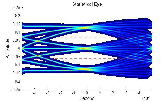
disp(statMetrics.eyeHeight);

    0.0875
    0.0875

For time-domain analysis, remove the ignore UI from the leading edge of the waveform and the Rx clock times contained in the AMIData structure.

%% Time domain results
% Pre-process time domain data
rxWaveOutIgnoreUI = rxWaveOut(ignoreUI*samplesPerBit+1:end); % Trim ignore UI
rxTDThresholds = parseThresholds(rxAMI.AMIData.GetWaveAMIOutput);
% Trim ignore bits from clock times, normalize to time 0 and shift 0.5 UI
% to account for IBIS-AMI output of edge times
clockStart = find(rxAMI.AMIData.ClockTimesOut>ignoreUI*symbolTime, 1, 'first');
rxClockTimes = rxAMI.AMIData.ClockTimesOut(clockStart:end)...
    - sampleInterval*(ignoreUI*samplesPerBit) + symbolTime/2;
% Plot time domain eye and  output key metrics
timeDomainMetrics = generateTimeDomainResults(...
    rxWaveOutIgnoreUI, symbolTime, sampleInterval, modulation, rxTDThresholds, rxClockTimes);

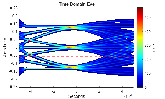
disp(timeDomainMetrics.eyeHeight);

    0.0940
    0.0920

Helper Functions

These functions help support the Processing Results section and are discussed inline here.

% Parse threshold data from AMI output string
function thresholds = parseThresholds(outputString)
    thresholds = [];
    searchPattern = 'PAM_Thresholds\s+"([^"]+)"';
    matches = regexp(outputString, searchPattern, 'tokens', 'once');
    if ~isempty(matches)
        thresholds = str2num(matches{1}); %#ok<ST2NM>
    end
end

% Plot statistical eye and generate metrics
function metrics = generateStatResults(pulse, symbolTime, samplesPerBit, modulation, targetBER, thresholds)
    [stateye,vh,th] = pulse2stateye(pulse, samplesPerBit ,modulation);
    th2 = (th*symbolTime)-(symbolTime/2);
    % Display figure with Stat eye
    figure;
    hold on
    siColorMap = serdes.utilities.SignalIntegrityColorMap;
    [mincval,maxcval]=serdes.internal.colormapToScale(stateye,siColorMap,1e-18);
    imagesc(th2,vh,stateye,[mincval,maxcval]);
    axis('xy');
    colormap(siColorMap)
    xlim([min(th2) max(th2)])
    xlabel('Second')
    ylabel('Amplitude')
    title('Statistical Eye')
    arrayfun(@(y) yline(y, '--', 'LineWidth', 1.5, 'Color', 'r'), thresholds)
    % Calculate metrics and add to metrics structure
    [metrics.eyeLinearity,...
        metrics.VEC,...
        metrics.contours,...
        metrics.bathtubs,...
        metrics.eyeHeight,...
        metrics.aHeight,...
        metrics.bestEyeHeight,...
        metrics.bestEyeHeightVoltage,...
        metrics.bestEyeHeightTime, ...
        metrics.bestEyeWidth,...
        metrics.bestEyeWidthTime,...
        metrics.bestEyeWidthVoltage,...
        metrics.vmidWidth,...
        metrics.vmidThreshold,...
        metrics.eyeAreas,...
        metrics.eyeAreaMetric,...
        metrics.COM] = ...
        serdes.utilities.calculatePAMnEye(...
        modulation, targetBER, min(th), max(th), min(vh), max(vh), stateye);
end

% Plot time domain eye and generate metrics
function metrics = generateTimeDomainResults(wave, symbolTime, sampleInterval, modulation, thresholds, clockTimes)
    eyeDiagramTD = eyeDiagramSI;
    eyeDiagramTD.SampleInterval = sampleInterval;
    eyeDiagramTD.SymbolTime = symbolTime;
    eyeDiagramTD.Modulation = modulation;
    eyeDiagramTD.SymbolThresholds = thresholds;
    eyeDiagramTD.SymbolsPerDiagram = 1;
    eyeDiagramTD(wave, clockTimes);
    figure
    eyeDiagramTD.plot;
    hold on
    title('Time Domain Eye')
    arrayfun(@(y) yline(y, '--', 'LineWidth', 1.5, 'Color', 'r'), thresholds)
    metrics.eyeHeight = eyeDiagramTD.eyeHeight;
    metrics.eyeWidth = eyeDiagramTD.eyeWidth;
end