Synchronous Machine GENROU

R2026b

GENROU synchronous generator model

Since R2026b

• 

Synchronous Machine GENROU block

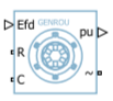
To add a block to a model, double-click the canvas and start typing the block name. Then, select the block from the list.

Libraries:
Simscape / Electrical / Electromechanical / Synchronous

Description

The Synchronous Machine GENROU block models a GENROU synchronous generator. GENROU synchronous generator models are widely used in power plant model verification and power system transient stability studies.

To model multiple GENROU synchronous machines using a single block, use the Vectorized Synchronous Machine GENROU block.

Synchronous Machine Initialization Using Load-Flow Target Values

If the block is in a network that is compatible with the frequency-time simulation mode, you can perform a load-flow analysis on the network. A load-flow analysis provides steady-state values that you can use to initialize the machine.

For more information, see Perform a Load-Flow Analysis Using Simscape Electrical and Frequency and Time Simulation Mode. For an example that shows how to initialize a synchronous machine using data from a load-flow analysis, see Synchronous Machine Initialization with Loadflow.

Equations

The block expresses the synchronous machine equations with respect to a rotating reference frame,

$${\theta }_e(t)=N{\theta }_r(t),$$

where:

• θ_e is the electrical angle.

• N is the number of pole pairs.

• θ_r is the rotor angle.

The Park transformation maps the synchronous machine equations to the rotating reference frame with respect to the electrical angle. This equation defines the Park transformation:

$$P_s=\frac{2}{3}\left[\begin{array}{ccc}\cos {\theta }_e& \cos ({\theta }_e-\frac{2\pi }{3})& \cos ({\theta }_e+\frac{2\pi }{3})\\ -\sin {\theta }_e& -\sin ({\theta }_e-\frac{2\pi }{3})& -\sin ({\theta }_e+\frac{2\pi }{3})\\ \frac{1}{2}& \frac{1}{2}& \frac{1}{2}\end{array}\right].$$

The block uses the Park transformation to define the per-unit synchronous machine equations. These equations define the d-axis and q-axis stator voltages:

$$\begin{array}{l}{v}_d=-{\omega }_r{{\psi }^{″}}_q-R_a{i}_d+{\omega }_r{X^{″}}_d{i}_q-\frac{{X^{″}}_d}{{\omega }_{base}}\frac{d{i}_d}{dt}\\ v_q={\omega }_r{{\psi }^{″}}_q-R_a{i}_q-{\omega }_r{X^{″}}_d{i}_d-\frac{{X^{″}}_d}{{\omega }_{base}}\frac{d{i}_q}{dt}\end{array}$$

In these equations:

• ω_r is the per-unit rotor rotational speed.

• ω_base is the electrical base speed.

• $${{\psi }^{″}}_d=\frac{{X^{\prime }}_d-{X^{″}}_d}{{X^{\prime }}_d-X_l}{{\psi }^{\prime }}_d+\frac{{X^{″}}_d-X_l}{{X^{\prime }}_d-X_l}{e^{\prime }}_q$$ is the d-axis flux linkage behind the subtransient reactance X^''_d.

• $${{\psi }^{″}}_q=-\frac{{X^{\prime }}_q-{X^{″}}_q}{{X^{\prime }}_q-X_l}{{\psi }^{\prime }}_q+\frac{{X^{″}}_q-X_l}{{X^{\prime }}_q-X_l}{e^{\prime }}_d$$ is the q-axis flux linkage behind the subtransient reactance X^''_q.

• ψ^'_d is the d-axis flux linkage behind the transient reactance X^'_d.

• ψ^'_q is the q-axis flux linkage behind the transient reactance X^'_q.

• R_a is the stator resistance.

• i_d is the d-axis stator current.

• i_q is the q-axis stator current.

• X^'_d is the d-axis transient reactance.

• X^''_d is the d-axis subtransient reactance.

• X^'_q is the q-axis transient reactance.

• X^''_q is the q-axis subtransient reactance.

• X_l is the stator leakage reactance.

• e^'_d is the d-axis voltage behind the transient reactance.

• e^'_q is the q-axis voltage behind the transient reactance.

These equations define the voltages behind the transient reactances:

$$\begin{array}{l}\frac{d{{\psi }^{\prime }}_d}{dt}=\frac{1}{{T^{″}}_{d0}}\left[{e^{\prime }}_q-{{\psi }^{\prime }}_d-\left({X^{\prime }}_d-X_l\right)i_d\right]\\ \frac{d{{\psi }^{\prime }}_q}{dt}=\frac{1}{{T^{″}}_{q0}}\left[{e^{\prime }}_d-{{\psi }^{\prime }}_q-\left({X^{\prime }}_q-X_l\right)i_q\right]\\ \frac{d{e^{\prime }}_d}{dt}=\frac{1}{{T^{\prime }}_{q0}}\left\{\left[i_q-\frac{{X^{\prime }}_q-{X^{″}}_q}{{\left({X^{\prime }}_q-X_l\right)}^2}\left({e^{\prime }}_d-{{\psi }^{\prime }}_q+\left({X^{\prime }}_q-X_l\right)i_q\right)\right]\left(X_q-{X^{\prime }}_q\right)+S\frac{X_q-X_l}{X_d-X_l}{{\psi }^{″}}_q-{e^{\prime }}_d\right\}\\ \frac{d{e^{\prime }}_q}{dt}=\frac{1}{{T^{\prime }}_{d0}}\left\{E_{fd}-\left[i_d+\frac{{X^{\prime }}_d-{X^{″}}_d}{{\left({X^{\prime }}_d-X_l\right)}^2}\left({e^{\prime }}_q-{{\psi }^{\prime }}_d+\left({X^{\prime }}_d-X_l\right)i_d\right)\right]\left(X_d-{X^{\prime }}_d\right)-S{{\psi }^{″}}_d-{e^{\prime }}_q\right\}\end{array}$$

In these equations:

• T^'_d0 is the d-axis transient open-circuit time constant.

• T^'_q0 is the q-axis transient open-circuit time constant.

• T^''_d0 is the d-axis subtransient open-circuit time constant.

• T^''_q0 is the q-axis subtransient open-circuit time constant.

• $$S=\frac{f\left({\psi }_{at}\right)}{{\psi }_{at}}$$ is the saturation factor:

  • $${\psi }_{at}=\sqrt{{{\psi }^{″}}_d{}^2+{{\psi }^{″}}_q{}^2}$$ is the air-gap flux linkage.

  • If you set the Magnetic saturation representation parameter to None, then the saturation factor is equal to zero.

  • If you set the Magnetic saturation representation parameter to Quadratic, Scaled quadratic, or Exponential, then the block calculates the saturation factor function, f, using the values of the Saturation factor S10 and Saturation factor S12 parameters.

  • If you set the Magnetic saturation representation parameter to Open-circuit lookup table, then the block calculates the saturation factor function using the values of the Per-unit air-gap voltage saturation data, Vag and Non-reciprocal per-unit field current saturation data, Ifd parameters.

This equation defines the per-unit field current in a non-reciprocal per-unit system:

$$I_{fd}=\left\{i_d+\frac{{X^{\prime }}_d-{X^{″}}_d}{{\left({X^{\prime }}_d-X_l\right)}^2}\left[{e^{\prime }}_q-{{\psi }^{\prime }}_d-\left({X^{\prime }}_d-X_l\right)i_d\right]\right\}\left(X_d-{X^{\prime }}_d\right)+S{{\psi }^{″}}_d+{e^{\prime }}_q.$$

This equation defines the rotor torque:

$$T{}_e={{\psi }^{″}}_d{i}_q-{{\psi }^{″}}_q{i}_d.$$

Plotting and Display Options

You can perform these plotting and display actions by clicking the button next to the associated parameter in the Utilities section:

• Base values — Display the machine per-unit base values in the MATLAB^® Command Window.

• Associated initial conditions — Display associated initial conditions in the MATLAB Command Window.

• Open-circuit saturation (pu) — Plot air-gap voltage, V_ag, versus field current, i_fd, both of which are per-unit measurements, in a MATLAB figure window. The plot contains an unsaturated and a saturated trace.

• Saturation factor (pu) — Plot the saturation factor, f, versus magnetic flux linkage, ψ_at, both of which are per-unit measurements, in a MATLAB figure window using the machine parameters. If you set the Magnetic saturation representation parameter to Quadratic, Scaled quadratic, or Exponential, then the block derives the saturation factor function from the value of the Saturation factor, S10 and Saturation factor, S12 parameters.

  If you set the Magnetic saturation representation to Open-circuit lookup table, then the block derives the saturation factor function from the value of the Non-reciprocal per-unit field current saturation data, Ifd and Per-unit air-gap voltage saturation data, Vag parameters.

• Power capability curves — Plot active power P versus reactive power Q, both of which are per-unit measurements, in a MATLAB figure window. The plot can contain multiple traces. Each trace corresponds to a maximum field circuit voltage measured per unit (non-reciprocal per-unit system). The plot shows the maximum reactive power that the generator produces when operating with a lagging power factor and the minimum reactive power that the generator absorbs when operating with a leading power factor.

Variables

To set the priority and initial target values for the block variables prior to simulation, use the Initial Targets section in the block dialog box or Property Inspector. For more information, see Set Priority and Initial Target for Block Variables.

For this block, the Initial Targets settings are visible only if, in the Initial Conditions section, you set the Initialization option parameter to Set targets for rotor angle and Park's transform variables.

Nominal values provide a way to specify the expected magnitude of a variable in a model. Using system scaling based on nominal values increases the simulation robustness. Nominal values can come from different sources, one of which is the Nominal Values section in the block dialog box or Property Inspector. For more information, see System Scaling by Nominal Values.

Ports

Input

Efd — Per-unit field voltage

physical signal

Physical signal port associated with the per-unit field voltage.

Output

pu — Machine per-unit measurements

physical signal vector

Physical signal vector port associated with the machine per-unit measurements. The vector elements are:

• Field voltage (field circuit base, Efd), pu_fd_Efd

• Field current (field circuit base, Ifd), pu_fd_Ifd

• Electrical torque, pu_torque

• Rotor velocity, pu_velocity

• Stator d-axis voltage, pu_vd

• Stator q-axis voltage, pu_vq

• Stator zero-sequence voltage, pu_v0

• Stator d-axis current, pu_id

• Stator q-axis current, pu_iq

• Stator zero-sequence current, pu_i0

• Rotor electrical angle, electrical_angle_out

To connect to this port, use the Synchronous Machine Measurement block.

Conserving

R — Machine rotor

mechanical

Mechanical rotational conserving port associated with the machine rotor.

C — Machine case

mechanical

Mechanical rotational conserving port associated with the machine case.

~ — Stator windings

three-phase electrical

Expandable three-phase electrical conserving port associated with the stator windings. For more information, see Three-phase ports.

Dependencies

To enable this port, set Electrical connection to Composite three-phase ports.

a — a-phase

electrical

Electrical conserving port associated with the a-phase.

Dependencies

To enable this port, set Electrical connection to Expanded three-phase ports.

b — b-phase

electrical

Electrical conserving port associated with the b-phase.

Dependencies

To enable this port, set Electrical connection to Expanded three-phase ports.

c — c-phase

electrical

Electrical conserving port associated with the c-phase.

Dependencies

To enable this port, set Electrical connection to Expanded three-phase ports.

Parameters

To edit block parameters interactively, use the Property Inspector. From the Simulink^® Toolstrip, on the Simulation tab, in the Prepare gallery, select Property Inspector.

Main

Electrical connection — Electrical connection

Composite three-phase ports (default) | Expanded three-phase ports

Option to model composite or expanded three-phase ports.

Rated apparent power — Rated apparent power

555e6 A*V (default) | positive scalar

Rated apparent power.

Rated voltage — RMS rated line-line voltage

24e3 V (default) | positive scalar

Root mean square (RMS) of the rated line-line voltage.

Rated electrical frequency — Nominal electrical frequency

60 Hz (default) | positive scalar

Nominal electrical frequency at which the block quotes the rated apparent power.

Number of pole pairs — Number of machine pole pairs

1 (default) | positive integer

Number of pole pairs that the machine has.

Rotor angle definition — Reference point for rotor angle measurement

Angle between the a-phase magnetic axis and the d-axis (default) | Angle between the a-phase magnetic axis and the q-axis

Reference point for the rotor angle measurement.

• Angle between the a-phase magnetic axis and the d-axis — The rotor d-axis and stator a-phase magnetic axis are aligned when the rotor angle is zero.

• Angle between the a-phase magnetic axis and the q-axis — The rotor q-axis and stator a-phase magnetic axis are aligned when the rotor angle is zero.

Impedances

Stator resistance, Ra — Resistance of stator

0.003 (default) | positive scalar

Resistance of the stator.

Stator leakage reactance, Xl — Leakage reactance of stator

0.15 (default) | positive scalar

Leakage reactance of the stator.

d-axis synchronous reactance, Xd — Direct-axis synchronous reactance

1.81 (default) | positive scalar

Direct-axis synchronous reactance.

q-axis synchronous reactance, Xq — Quadrature-axis synchronous reactance

1.76 (default) | positive scalar

Quadrature-axis synchronous reactance.

d-axis transient reactance, Xd' — Direct-axis transient reactance

0.3 (default) | positive scalar

Direct-axis transient reactance.

q-axis transient reactance, Xq' — Quadrature-axis transient reactance

0.65 (default) | positive scalar

Quadrature-axis transient reactance.

d-axis subtransient reactance, Xd'' — Direct-axis subtransient reactance

0.23 (default) | positive scalar

Direct-axis subtransient reactance.

q-axis subtransient reactance, Xq'' — Quadrature-axis subtransient reactance

0.25 (default) | positive scalar

Quadrature-axis subtransient reactance.

Time Constants

d-axis transient open-circuit, Td0' — Direct-axis transient open-circuit

8 s (default) | positive scalar

Direct-axis transient open-circuit time constant. The value of this parameter must be greater than the value of the d-axis subtransient open-circuit, Td0'' parameter.

d-axis subtransient open-circuit, Td0'' — Direct-axis subtransient open-circuit

0.03 s (default) | positive scalar

Direct-axis subtransient open-circuit time constant. The value of this parameter must be less than the value of the d-axis transient open-circuit, Td0' parameter.

q-axis transient open-circuit, Tq0' — Quadrature-axis transient open-circuit

1 s (default) | positive scalar

Quadrature-axis transient open-circuit time constant. The value of this parameter must be greater than the value of the q-axis subtransient open-circuit, Tq0'' parameter.

q-axis subtransient open-circuit, Tq0'' — Quadrature-axis subtransient open-circuit

0.07 s (default) | positive scalar

Quadrature-axis subtransient open-circuit time constant. The value of this parameter must be less than the value of the q-axis transient open-circuit, Tq0' parameter.

Saturation

Magnetic saturation representation — Magnetic saturation representation

None (default) | Quadratic | Scaled quadratic | Exponential | Open-circuit lookup table

Option to represent the magnetic saturation of the block:

• None — The block does not model the magnetic saturation.

• Quadratic — The block models the magnetic saturation by using a quadratic function.

• Scaled quadratic — The block models the magnetic saturation by using a scaled function.

• Exponential — The block models the magnetic saturation by using an exponential function.

• Open-circuit lookup table — The block models the magnetic saturation by using per-unit non-reciprocal field current and per-unit air-gap voltage saturation data.

Saturation factor, S10 — Saturation factor, S10

0.005 (default) | nonnegative scalar

Saturation factor that corresponds to 1.0 per-unit terminal voltage. The value of this parameter must be less than the value of the Saturation factor, S12 parameter. If you set the Magnetic saturation representation parameter to Exponential, the value of this parameter must be greater than zero.

Dependencies

To enable this parameter, set Magnetic saturation representation to Quadratic, Scaled quadratic, or Exponential.

Saturation factor, S12 — Saturation factor, S12

0.08 (default) | positive scalar

Saturation factor that corresponds to 1.2 per-unit terminal voltage. The value of this parameter must be greater than the value of the Saturation factor, S10 parameter.

Dependencies

To enable this parameter, set Magnetic saturation representation to Quadratic, Scaled quadratic, or Exponential.

Non-reciprocal per-unit field current saturation data, Ifd — Non-reciprocal per-unit field current saturation data

[0, .8, 1.26, 2.29, 2.97] (default) | vector of nonnegative values

Nonreciprocal field current, I_fd, data that populates the lookup table for air-gap voltage, V_ag, versus field current. The value of this parameter must be a vector of at least five elements.

Dependencies

To enable this parameter, set Magnetic saturation representation to Open-circuit lookup table.

Per-unit air-gap voltage saturation data, Vag — Per-unit air-gap voltage saturation data

[0, .8, 1.08, 1.31, 1.4] (default) | vector of nonnegative values

Air-gap voltage, V_ag, data that populates the lookup table for air-gap voltage versus field current, i_fd. The value of this parameter must be a vector of at least five elements.

Dependencies

To enable this parameter, set Magnetic saturation representation to Open-circuit lookup table.

Initial Conditions

Initialization option — Option for specifying values at start of simulation

Set real power, reactive power, terminal voltage, and terminal phase (default) | Set targets for rotor angle and Park's transform variables | Set targets for load flow variables

Option for specifying values for certain parameters and variables at the start of simulation:

• Set real power, reactive power, terminal voltage, and terminal phase — Set an operating point regardless of the connected network.

• Set targets for rotor angle and Park's transform variables — Specify the priority and initial target values for block variables before simulation by using the Variables settings. For more information, see Set Priority and Initial Target for Block Variables.

• Set targets for load flow variables — In the Initial Conditions settings, select a bus type and specify the related parameters for a load-flow analysis.

Source type — Voltage source model

Swing bus (default) | PV bus | PQ bus

Type of voltage source that the block models.

Dependencies

To enable this parameter, set Initialization option to Set targets for load flow variables.

Terminal voltage magnitude — Magnitude of terminal voltage

24e3 V (default) | positive scalar

Magnitude of the terminal voltage.

Dependencies

To enable this parameter, set Initialization option to Set real power, reactive power, terminal voltage, and terminal phase.

Alternatively, set Initialization option to Set targets for load flow variables and Source type to Swing bus or PV bus.

Terminal voltage angle — Angle of terminal voltage

0 deg (default) | scalar

Angle of the terminal voltage.

Dependencies

To enable this parameter, set Initialization option to Set real power, reactive power, terminal voltage, and terminal phase.

Alternatively, set Initialization option to Set targets for load flow variables and Source type to Swing bus.

Active power generated — Generated active power

500e6 V*A (default) | nonnegative scalar

Active power that the machine generates.

Dependencies

To enable this parameter, set Initialization option to Set real power, reactive power, terminal voltage, and terminal phase.

Alternatively, set Initialization option to Set targets for load flow variables and Source type to PV bus or PQ bus.

Reactive power generated — Generated reactive power

0 V*A (default) | scalar

Reactive power that the machine generates.

Dependencies

To enable this parameter, set Initialization option to Set real power, reactive power, terminal voltage, and terminal phase.

Alternatively, set Initialization option to Set targets for load flow variables and Source type to PQ bus.

Minimum terminal voltage magnitude (pu) — Minimum terminal voltage magnitude

0.95 (default) | positive scalar

Minimum per-unit magnitude of the steady-state voltage.

Dependencies

To enable this parameter, set Initialization option to Set targets for load flow variables and Source type to PQ bus.

Phase search range at terminals — Search range of phase angle at terminals

[-inf, inf] deg (default) | vector of two elements

Search range of the phase angle at the terminals.

Dependencies

To enable this parameter, set Initialization option to Set targets for load flow variables and Source type to PV bus or PQ bus.

Parasitic conductance to electrical reference — Parasitic conductance to electrical reference

1e-6 S (default) | nonnegative scalar

Parasitic conductance to the electrical reference. If you connect the machine to a delta-wound transformer, the value must be greater than zero.

Dependencies

To enable this parameter, set Initialization option to Set targets for load flow variables.

Utilities

Base values — Display machine per-unit base values

button

Display the machine per-unit base values in the MATLAB Command Window.

Associated initial conditions — Display associated initial conditions

button

Display the associated initial conditions in the MATLAB Command Window.

Open-circuit saturation (pu) — Plot air-gap voltage against field current

button

Plot the air-gap voltage, V_ag, against the field current, i_fd, both of which are per-unit measurements, in a MATLAB figure window.

Saturation factor (pu) — Plot saturation factor against magnetic flux linkage

button

Plot the saturation factor, f, against the magnetic flux linkage, ψ_at, both of which are per-unit measurements, in a MATLAB figure window using the machine parameters.

Power capability curves — Plot active power against reactive power

button

Plot the active power P against the reactive power Q, both of which are per-unit measurements, in a MATLAB figure window.

References

[1] Sauer, Peter W., and M. A. Pai. "Power System Dynamics and Stability". Prentice Hall, 1998.

Extended Capabilities

C/C++ Code Generation
Generate C and C++ code using Simulink® Coder™.

Version History

Introduced in R2026b