MPC with Disturbance Compensator for a MIMO Plant

Since R2026a

This example uses:

This example shows how to design a Model Predictive Controller (MPC) for a multivariable (MIMO) plant by first using a Disturbance Compensator block to cancel unknown dynamics and disturbances. With this approach:

The original plant is transformed into a simple nominal model (e.g., a double integrator).
MPC is designed on the nominal model, avoiding the need for detailed plant identification.
The resulting controller retains the advantages of MPC (constraint handling and optimization) while improving robustness to model uncertainty.

Motivation

Model Predictive Control (MPC) is powerful for handling multivariable systems with constraints, but it requires an accurate prediction model. In practice, modeling errors and unknown disturbances degrade MPC performance and make controller design difficult. The key idea of this example is:

Use a Disturbance Compensator to cancel uncertainties and disturbances.
After compensation, the effective plant is reduced to a nominal simple model.
Design MPC on this nominal model is easier and more robust.

This example also compares the following two designs:

Benchmark MPC (assuming plant model is known).
MPC with Disturbance Compensator.

Setup Plant Model

The plant is taken from the Design ADRC for Multi-Input Multi-Output Plant example. The plant is a model of a pilot-scale distillation column. This model has two inputs: the flux flow rate $u_{1}$ and the steam flow rate $u_{2}$ . The model has two outputs: the purity of light product $y_{1}$ and the purity of heavy product $y_{2}$ . The model also contains unknown disturbances.

Define the plant transfer function. The following transfer function matrix is the plant model used in the "Design ADRC for Multi-Input Multi-Output Plant" example.

s = tf('s');
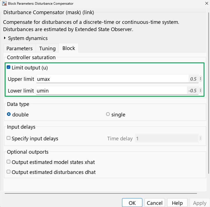
G = [12.8/(16.7*s+1),-18.9/(21*s+1);6.6/(10.9*s+1),-19.4/(14.4*s+1)];

The controller objective is to keep the outputs at desired values $r_{1} = 0$ and $r_{2} = 1$ . Considering the physical limitations of the plant dynamics, the inputs to the plant are constrained to the range $[- 0.5, 0.5]$ .

umin = -0.5;
umax = 0.5;

Benchmark MPC

Design an MPC controller for the plant model.

Ts = 1; % sample time
mpc1 = mpc(G,Ts);

-->"PredictionHorizon" is empty. Assuming default 10.
-->"ControlHorizon" is empty. Assuming default 2.
-->"Weights.ManipulatedVariables" is empty. Assuming default 0.00000.
-->"Weights.ManipulatedVariablesRate" is empty. Assuming default 0.10000.
-->"Weights.OutputVariables" is empty. Assuming default 1.00000.

Specify weights for the MPC controller.

mpc1.Weights.ManipulatedVariablesRate = 0.7389*[1,1];
mpc1.Weights.OutputVariables = 0.1353*[1,1];

You can adjust the weights of the controller to tune the performance. For more information, see Tune Weights (Model Predictive Control Toolbox).

Specify the limits for the MPC controller.

mpc1.MV(1).Min = umin;
mpc1.MV(1).Max = umax;
mpc1.MV(2).Min = umin;
mpc1.MV(2).Max = umax;

Disturbance Compensator

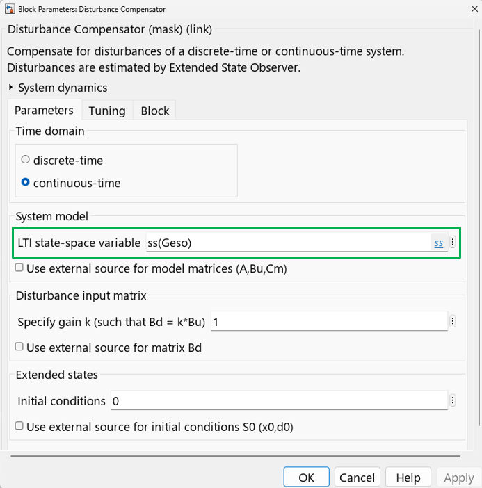
The Disturbance Compensator block is designed based upon a nominal model. The plant is approximated by a diagonal nominal model with each channel behaving like a single integrator.

b1 = 0.75;
b2 = -1.3;
Geso = [b1/s,0;0,b2/s];

For more information on how to obtain the nominal model $G_{e s o}$ , see the Design ADRC for Multi-Input Multi-Output Plant example. The nominal model can be specified in the Disturbance Compensator block as follows.

Specify the observer bandwidth for the "Disturbance Compensator" block.

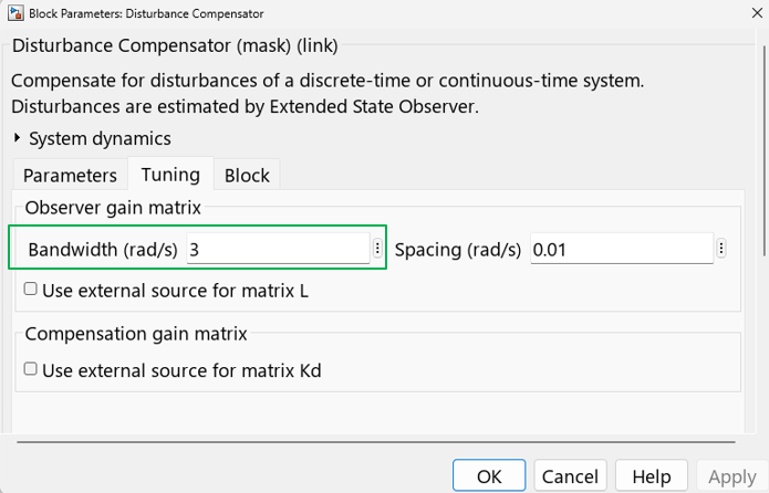
You can tune the observer bandwidth so that the outputs $y$ can match the response of benchmark MPC controller $y_{b e n c h m a r k}$ .

Specify the controller limits for the "Disturbance Compensator" block.

MPC on Nominal Model

Design an MPC controller for the nominal model.

mpc2 = mpc(Geso,Ts);

-->"PredictionHorizon" is empty. Assuming default 10.
-->"ControlHorizon" is empty. Assuming default 2.
-->"Weights.ManipulatedVariables" is empty. Assuming default 0.00000.
-->"Weights.ManipulatedVariablesRate" is empty. Assuming default 0.10000.
-->"Weights.OutputVariables" is empty. Assuming default 1.00000.

Specify weights for the MPC controller.

mpc2.Weights.ManipulatedVariablesRate = 0.7389*[1,1];
mpc2.Weights.OutputVariables = 0.1353*[1,1];

For fair comparison, the same weights are used for both MPC designs. You can also tune the weights so that the outputs $y$ can match the response of benchmark MPC controller $y_{b e n c h m a r k}$ .

Simulation Results

Both designs are simulated in one Simulink model.

mdl = 'MPC_With_DisturbanceCompensator';
open_system(mdl)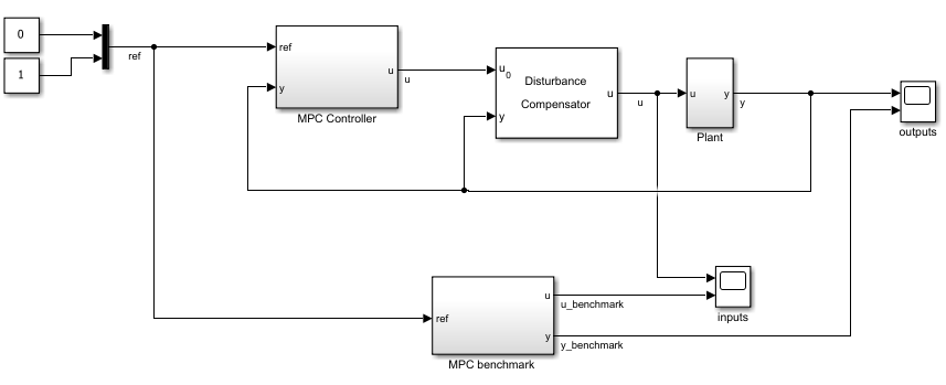

The model has an external disturbance from 50 to 100 seconds. Run the model to 150 seconds.

T = 150;
sim(mdl);

-->Converting the "Model.Plant" property to state-space.
-->Converting model to discrete time.
   Assuming no disturbance added to measured output #1.
   Assuming no disturbance added to measured output #2.
-->"Model.Noise" is empty. Assuming white noise on each measured output.
-->Converting the "Model.Plant" property to state-space.
-->Converting model to discrete time.
-->Integrator added as output disturbance model for measured output #1.
-->Integrator added as output disturbance model for measured output #2.
-->"Model.Noise" is empty. Assuming white noise on each measured output.

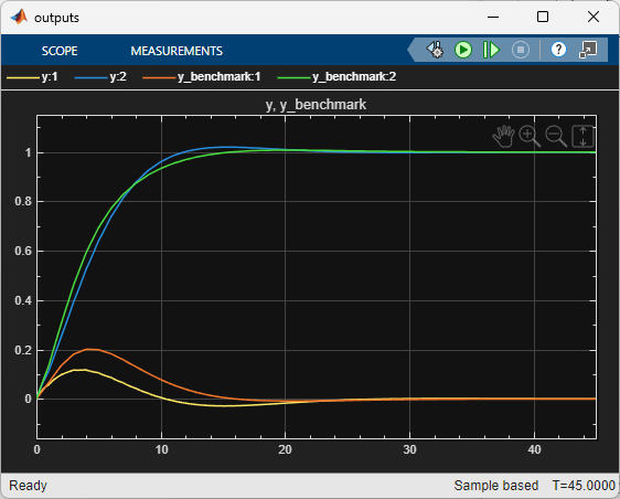
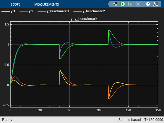
View the outputs of the plant using the scope.

open_system(mdl + "/outputs")

The design with disturbance compensation shows improved disturbance rejection compared to the benchmark MPC. The outputs converge more quickly to their reference values, though this comes at the cost of larger control effort.

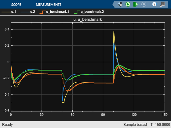
View the inputs of the plant using the scope.

open_system(mdl + "/inputs")

Conclusions

This example shows that by combining a Disturbance Compensator with MPC, one can design controllers based on a simple nominal integrator model while still achieving good reference tracking and disturbance rejection. The main benefit is avoiding detailed plant modeling, which simplifies design and tuning.