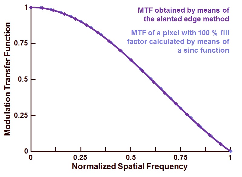
FFT with normalized spatial frequency for image sensor MTF
38 visualizaciones (últimos 30 días)
Mostrar comentarios más antiguos
I'm attempting to use the slanted edge method to calculate the MTF for a camera system according to Harvest Imaging (https://harvestimaging.com/blog/?p=1328), and struggling to plot the result correctly. The method involves taking the Fourier transform of a line spread function and plotting it from DC to the sampling frequency. I have chosen the sampling frequency to equal 2, since that is the minimum number of pixels required to record contrast. Here is my code:
LSF = [];
LSF(1:250) = 0;
LSF(51:70) = 140;
Fs = 2; % Sampling frequency (pixels/lp)
T = 1/Fs; % Sampling period (lp/pixel)
L = length(LSF); % Length of signal (length of line in pixels)
P2 = abs(fft(LSF/L));
P1 = P2(1:L/2+1);
P1(2:end-1) = 2*P1(2:end-1);
f = Fs*(0:(L/2))/L;
nP1 = P1-min(P1);
nP1 = nP1./max(nP1);
plot(f,nP1,'linewidth',3)
title('MTF')
xlabel('Normalized Spatial Frequency')
According to the example, I should reach my first minimum of the sinc function at x=1

But, I appear to be off by a factor of 10.

Can anyone point out where I'm going wrong? I'm sure it's a simple fix.
Thanks much!
7 comentarios
Ali Madani
el 22 de Oct. de 2020
Hi Ben, did you figure out how to normalized the x-axis? I've been having the same question and cannot figure out how to do this.
Respuestas (1)
Jack
el 22 de Abr. de 2020
Editada: Jack
el 22 de Abr. de 2020
Hi Ben,
You are off by a factor of 10 because there are 10 samples in one of your 'pixels'. The result of the FT is in cycles/set, which can also be expressed in other units as shown below (see here for a detailed explanation). I used similar figures to yours that however result in the sinc having samples at MTF nulls.
Jack
n = 256; %samples per set
px = 16; %samples per pixel
LSF = zeros(1,n);
LSF(1:px)=140; %the pixel has intensity 140
MTF = 1/sum(LSF) * abs(fft(LSF));
f = 0:n-1; %cycles per set
figure; plot(f,MTF); %cycles per set
xlabel('cycles/set'); ylabel('MTF')
figure; plot(f/n,MTF); %cycles per sample
xlabel('cycles/sample'); ylabel('MTF')
figure; plot (f/n*px,MTF) %cycles per pixel
xlabel('cycles/pixel'); ylabel('MTF'); xlim([0 1])
0 comentarios
Ver también
Categorías
Más información sobre Fourier Analysis and Filtering en Help Center y File Exchange.
Productos
Community Treasure Hunt
Find the treasures in MATLAB Central and discover how the community can help you!
Start Hunting!

