Resultados de

The MATLAB One-Button Game Mini Hack runs from November 2nd through November 29th, 2026! The challenge is to make a game that can be played with one button. I thought this would be a good opportunity to share some of the graphics and programming ideas behind Arcade, a collection of 15 games I developed in MATLAB using Claude Code and the MATLAB MCP Server.
Before the 2024 MATLAB Shorts Mini Hack, Tim Marston published his walkthrough of Little Nemo's airship. I learned a lot from Tim's article, and it inspired me to enter the contest. I hope that sharing some of what goes into these games might encourage a few more people to give it a try this time around as well.
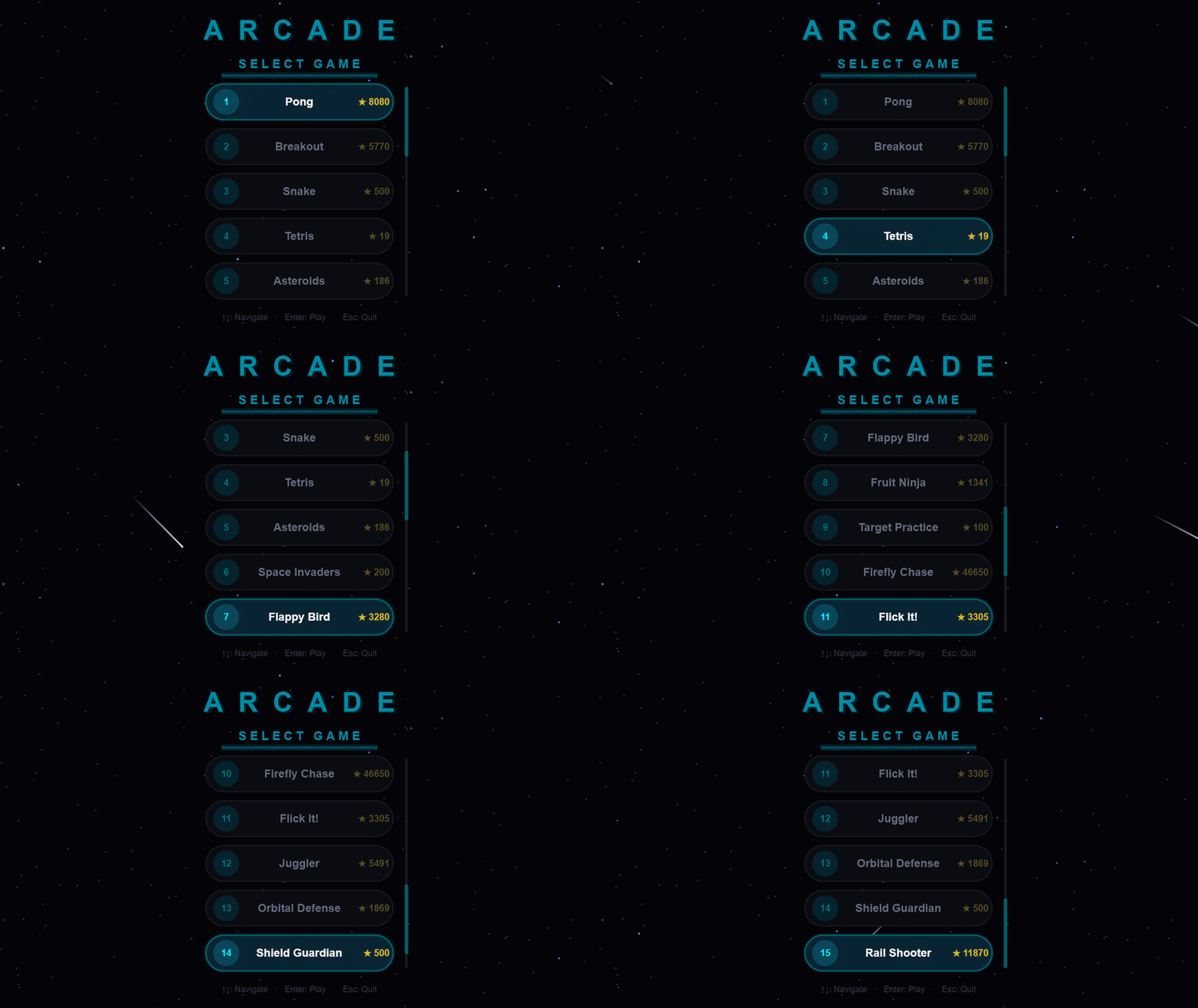
You can download Arcade from File Exchange or GitHub, add the project folder to the MATLAB search path, and run:
Arcade();
Creating and updating graphics
Arcade sports neon-styled graphics. This is accomplished by layering ordinary MATLAB graphics against a dark background. The bright colors used come from the shared GameBase palette, which enables the different games to keep a consistent appearance and accounts for quite a bit of that look.
In Pong, the ball is made by drawing a colored dot, a semitransparent scatter marker and a smaller white dot at the same position. The ball and trail change from cyan through green, gold and red as the ball speeds up, while the center stays white. Against the dark background, these simple shapes give us the bright center and surrounding glow.
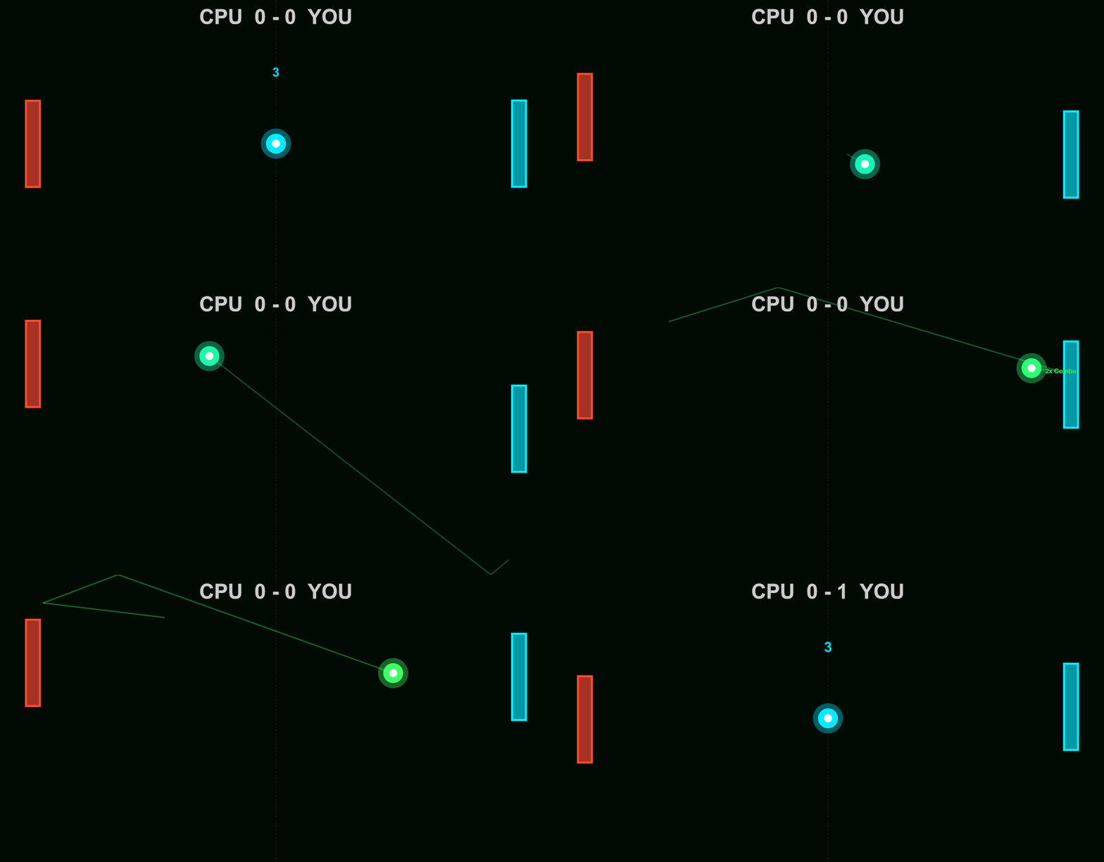
arcadeBallDemo();
worldSize = [854, 480];
position = worldSize / 2;
cyan = [0, 0.92, 1];
radiusParameter = max(3, round(min(worldSize) * 0.035));
baseCoreSize = 2 * radiusParameter;
baseDotSize = 5 * radiusParameter;
baseGlowArea = pi * (1.25 * radiusParameter)^2;
coloredDot = line(ax, NaN, NaN, ...
Marker=".", MarkerSize=baseDotSize, LineStyle="none", Color=[cyan, 0.15]);
glow = scatter(ax, position(1), position(2), baseGlowArea, cyan, "filled", ...
MarkerFaceAlpha=0.4);
core = line(ax, position(1), position(2), ...
Marker=".", MarkerSize=baseCoreSize, LineStyle="none", Color=[1, 1, 1, 1]);
ballLayers = {coloredDot, glow, core};
Here's how the ball looks as each layer is added:
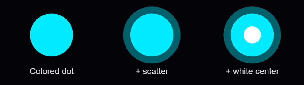
Setting NextPlot="add" preserves the existing graphics as we add the layers. Specifying the axes limits by using XLim and YLim keeps the view in place as the ball moves.
Each drawing call returns a handle to its object. With those handles stored in ballLayers, moving the ball involves assigning its new position to the existing objects:
for layerIndex = 1:numel(ballLayers)
ballLayers{layerIndex}.XData = position(1);
ballLayers{layerIndex}.YData = position(2);
end
drawnow
MathWorks' graphics-performance guidance recommends retaining graphics and updating the properties that change. Pong also checks whether its scores have changed before assigning new score text. Its trail uses preallocated position buffers, wrapping around as new positions arrive, and two retained lines display that history as a broad dim stroke with a narrower bright stroke.
Handling inputs using callback functions
The ball example responds to mouse presses through a callback function. After creating the scene, it assigns a function handle to the figure's WindowButtonDownFcn callback property:
fig.WindowButtonDownFcn = @reverseVerticalDirection;
MATLAB executes the callback function when a mouse button is pressed in the window. In the example, it is nested inside the local animateBall function:
function reverseVerticalDirection(~, ~)
velocity(2) = -velocity(2);
end
The two arguments supplied by MATLAB are the source object and event data. The ~ placeholders indicate that this function doesn't use them. As a nested function, it can access velocity in the enclosing function. Each mouse press reverses the shared vertical velocity, which the next loop iteration uses to move the ball.
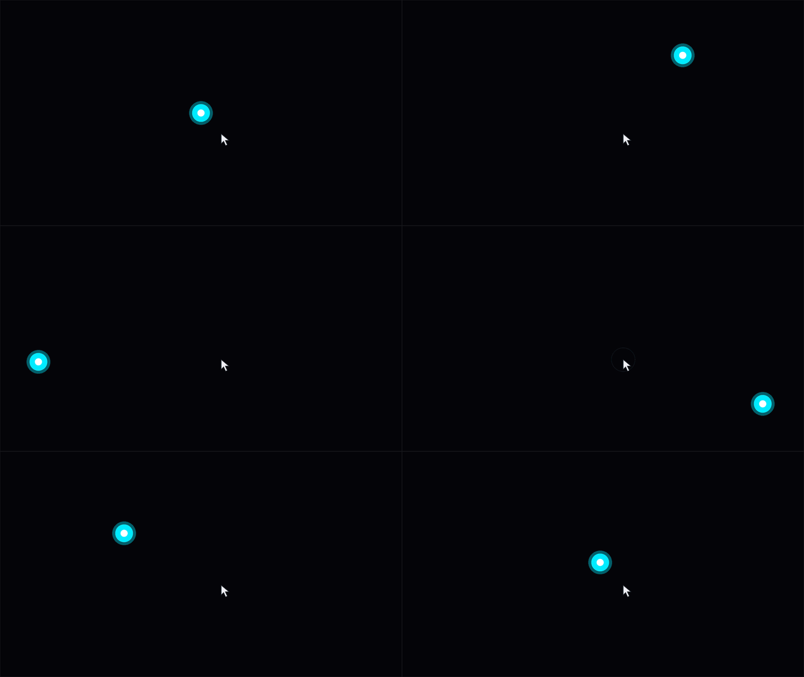
Arcade routes input through methods on the launcher. Its figure's KeyPressFcn callback property is assigned as follows, where obj is the launcher instance:
obj.Fig.KeyPressFcn = @(~, event) obj.onKeyPress(event);
The anonymous function forwards the event data to onKeyPress, where its Key property identifies the key. The launcher handles its own controls and passes appropriate input to the active game. Button release and scrolling have their own callback functions.
Mouse movement can control a paddle or aim a shot. To track the pointer as it moves within the figure, Arcade assigns a callback function to WindowButtonMotionFcn:
obj.Fig.WindowButtonMotionFcn = @(~, ~) obj.onMouseMove();
function onMouseMove(obj)
pointer = obj.Ax.CurrentPoint;
obj.MousePos = pointer(1, 1:2);
end
The axes' CurrentPoint gives the pointer position in game coordinates. MATLAB accounts for the axes' position and size, so the same code works when the playfield is resized or surrounded by margins.
On each game update, the launcher passes the stored position to the active game's onUpdate method. In Pong, obj now refers to the game instance. Once the incoming pos is available, its vertical coordinate determines the player's paddle position:
yLimits = obj.DisplayRange.Y;
if ~any(isnan(pos))
obj.PlayerPaddleY = max(yLimits(1) + obj.PaddleHalfH, ...
min(yLimits(2) - obj.PaddleHalfH, pos(2)));
end
The min and max calls keep the paddle's center at least half a paddle height from either edge. Moving the pointer into a margin therefore leaves the whole paddle inside the playfield. The graphics update then applies that position to the existing paddle patches.
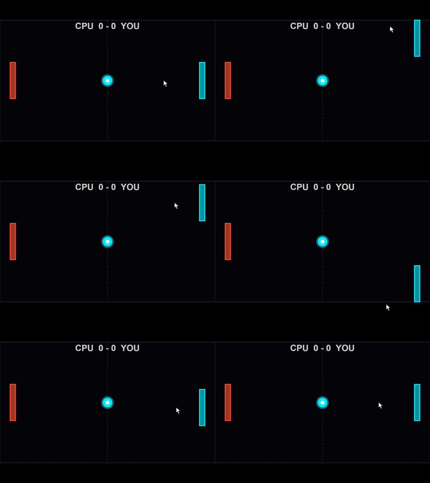
The animation loop's drawnow displays pending graphics changes and processes pending callbacks. Keeping callback functions short allows control to return to the loop promptly.
Animating visual effects
When the orb is launched in Flick It!, a call to spawnHitEffect creates a ring and rays that expand and fade. The launcher advances these shared effects alongside the active game.
In arcadeEffectsDemo.m, each click creates a burst at the mouse position, allowing several bursts to expand and fade together. To try it out, download the function, add its folder to the MATLAB path, and run:
arcadeEffectsDemo();
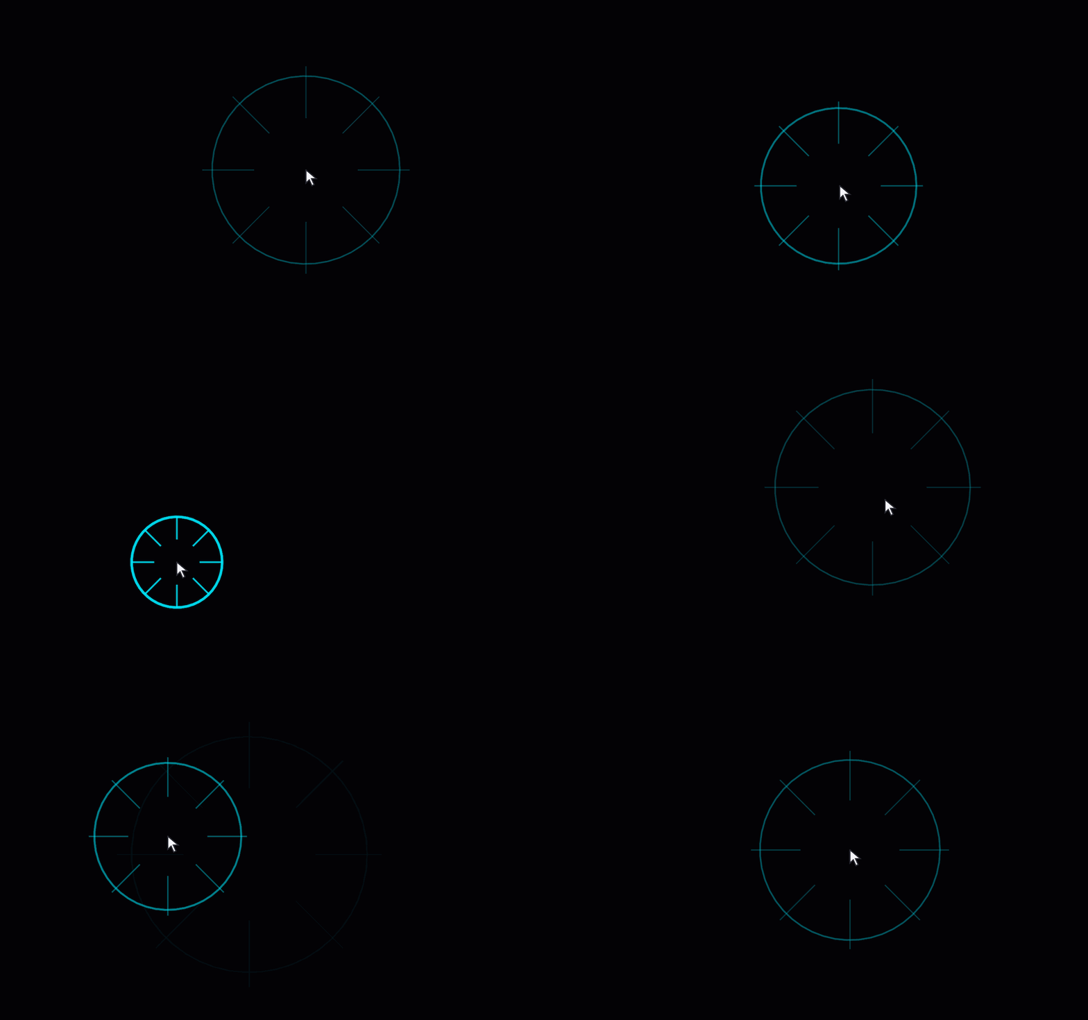
The nested callback function combines mouse-press handling with the mouse-position tracking introduced earlier. Here's the part that creates and stores a new burst:
fig.WindowButtonDownFcn = @createManualImpact;
function createManualImpact(~, ~)
point = ax.CurrentPoint;
position = point(1, 1:2);
if any(~isfinite(position)) || any(position < 0 | position > worldSize)
return
end
[newRing, newRays] = createEffect(position);
activeEffects(end+1) = struct('Ring', newRing, 'Rays', newRays, ...
'Center', position, 'AgeSeconds', 0, 'LastTime', toc(animationClock));
end
The bounds check ignores clicks outside the playfield. createEffect creates the lines, and activeEffects stores their handles, center and timing state. The animation loop updates each burst independently, allowing further clicks while earlier bursts are still expanding.
We can drive the geometry, transparency and line width from a common progress value: 0 when the burst begins and 1 at the end of its lifetime. Inside the function, the ring is updated as follows:
progress = ageSeconds / lifetimeSeconds;
eased = 1 - (1-progress)^2;
opacity = max(0, 1-1.5*eased);
ringRadius = radiusParameter * (1+2.5*eased);
ring.XData = center(1) + ringRadius*ringCos;
ring.YData = center(2) + ringRadius*ringSin;
ring.Color = [cyan, 0.8 * opacity];
ring.LineWidth = max(0.5, 3*(1-eased));
The ease-out expression starts the expansion quickly and slows it down toward the end. The burst fades out before its nominal lifetime finishes. ringCos and ringSin hold the circle's fixed directions, calculated before the loop. Arcade controls the transparency of these lines by assigning an RGBA value to Color, with alpha as the fourth component, ranging from 0 (clear) to 1 (fully opaque).
The row vectors rayCos and raySin contain the eight ray directions. Each ray joins the inner and outer radii, which increase as the burst expands:
innerRadius = radiusParameter * (0.5+1.5*eased);
outerRadius = radiusParameter * (1+3*eased);
for rayIndex = 1:numel(rays)
rays(rayIndex).XData = center(1) + [innerRadius, outerRadius]*rayCos(rayIndex);
rays(rayIndex).YData = center(2) + [innerRadius, outerRadius]*raySin(rayIndex);
rays(rayIndex).Color = [cyan, 0.6 * opacity];
rays(rayIndex).LineWidth = max(0.5, 2*(1-eased));
end
The lines are created when the burst begins, updated throughout its lifetime and deleted when it expires.
Display scaling: Keeping the scene in proportion
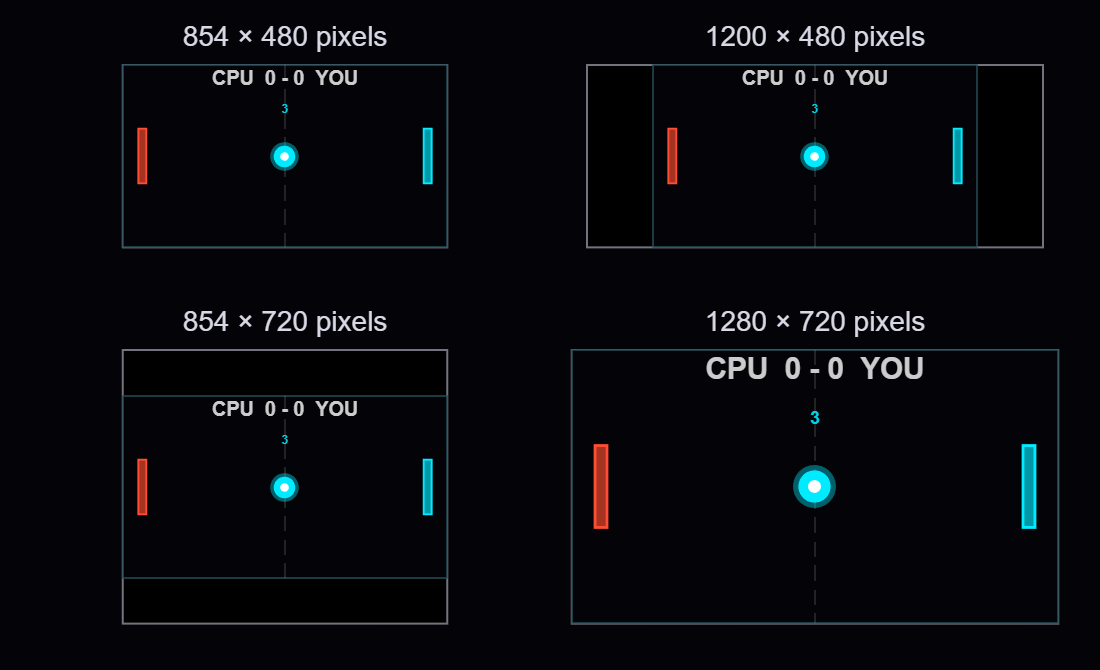
Try making the ball example's window wider while keeping its height the same. Space appears beside the playfield, and the ball still travels between the same boundaries. The example's reference window is 854 by 480 pixels, matching worldSize numerically. Resizing scales the playfield on the screen while the game's coordinate system remains unchanged.
The figure and axes use Units="pixels". Taking the min of the width and height ratios relative to the reference window gives the largest scale factor that fits in both directions. Applying that same scale to both dimensions preserves the playfield's 16:9 aspect ratio.
For a 1200-by-480 window, the height limits the scale to 1. The fitted area remains 854 by 480, leaving (1200-854)/2 = 173 pixels on each side. In a 1280-by-720 window, the playfield grows to approximately 1.5 times its reference width and height. Here are four window sizes at a common page scale:
MATLAB already scales graphics defined in data coordinates as the axes resize. For example, a paddle drawn with patch grows with the axes. In the example, marker sizes, font sizes and line widths use points, while scatter sizes use points squared.

To make a circle twice as wide, we need four times its area. Doubling SizeData multiplies its width by only √2:
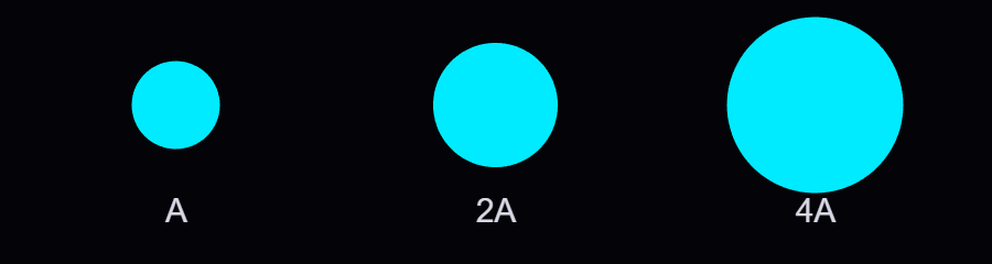
fig.SizeChangedFcn = @fitScene;
The nested fitScene callback function combines the axes calculation with these size updates:
function fitScene(~, ~)
if ~isgraphics(ax)
return
end
availableSize = max(fig.Position(3:4), [1, 1]);
displayScale = min(availableSize ./ worldSize);
fittedSize = worldSize * displayScale;
ax.Position = [(availableSize - fittedSize)/2 + 1, fittedSize];
% Always derive sizes from their reference values
core.MarkerSize = baseCoreSize * displayScale;
coloredDot.MarkerSize = baseDotSize * displayScale;
glow.SizeData = baseGlowArea * displayScale^2;
instruction.FontSize = baseFontSize * displayScale;
playfield.LineWidth = 0.5 * displayScale;
end
The first two entries of ax.Position set the left and bottom position, splitting the unused space equally between opposite sides. The last two give the fitted width and height. The axes limits remain unchanged, so movement and collision calculations keep using the same game coordinates.
At scale 1.5, the marker sizes are multiplied by 1.5 and the scatter area by 2.25. The updated sizes are calculated from their stored reference values. A 34-point reference marker becomes 51 points at scale 1.5, then 68 points at scale 2.
You can also use Units="normalized" to size and position the axes relative to the figure. Arcade's axes setup uses [0 0 1 1] to allocate the full available area:
obj.Ax = axes(obj.Fig, "Units", "normalized", "Position", [0 0 1 1]);
obj.Ax.XLim = obj.DisplayRange.X;
obj.Ax.YLim = obj.DisplayRange.Y;
Arcade's resize method obtains the available dimensions in pixels with getpixelposition and calculates the same display scale. It uses pbaspect to preserve the playfield's aspect ratio. MATLAB fits the playfield within the available space, leaving margins where needed:
axPx = getpixelposition(obj.Ax);
newPs = min(axPx(3) / 854, axPx(4) / 480);
gameAR = diff(obj.DisplayRange.X) / diff(obj.DisplayRange.Y);
pbaspect(obj.Ax, [gameAR 1 1]);
For Arcade, I also wanted markers, text and line widths to grow proportionally with the playfield. MATLAB also supports automatic resizing for text through FontUnits="normalized", which expresses font size as a fraction of the axes plot box height. This works well for text in a playfield with a fixed aspect ratio. Arcade's shared resize helper modifies current property values, using the ratio of the new scale to the previous scale; for example, moving from 51 to 68 points requires multiplying by 2/1.5. The function applies a common display scale to text, markers and line widths, in order to preserve their relative sizes as the window is resized.
FPS scaling: Let elapsed time determine the motion
Suppose that the ball moves 5 game units on each update. At 60 updates per second it travels 300 units in a second, but at 30 it travels only 150. Calculating the state, drawing and processing input all contribute to the time between updates, so we need to measure that interval to maintain a consistent speed.
Gianluca Carnielli discusses the relationship between time and animation frames in Animating Science: Creating Time-Sensitive Animations with MATLAB. In his example, he explains how to create a frame-based animation from time-based coordinates, by choosing the video’s duration and frame rate, calculating the simulation timestep between two consecutive frames, and resampling the coordinates using retime.
In a live game, we process player actions and calculate each new state using the time elapsed since the previous update. Arcade expresses many motion parameters per reference interval, using 60 frames per second (FPS) as its reference frequency. An elapsed time of 1/60 seconds represents 1 reference interval, while 1/30 seconds represents 2. In the example, we define the velocity and reference frequency before the loop and start the clock with tic once the initial scene is displayed:
velocity = [5, 3]; % Game units per reference interval
referenceFPS = 60; % Reference intervals per second
animationClock = tic;
previousTime = 0;
currentTime = toc(animationClock);
dtSeconds = min(currentTime - previousTime, 0.1);
previousTime = currentTime;
dtScale = dtSeconds * referenceFPS;
position = position + velocity * dtScale;
Here dtSeconds is in seconds, and dtScale counts reference intervals. A horizontal velocity of 5 now gives a movement of 10 game units over 1/30 second. Taking 30 steps of 10 units covers the same 300 units as 60 steps of 5 units. The samples are farther apart, so the motion can look less smooth:
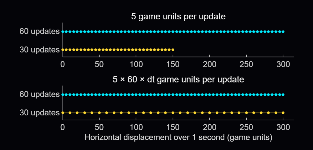
The min(..., 0.1) caps a single represented interval at 0.1 seconds (10 FPS) to limit jumps after a stall. If an update arrives after 0.5 seconds, the code advances only 0.1 seconds, and the remaining 0.4 seconds are discarded.
The reference frequency is 60 FPS; the actual update rate depends on execution. We could also use game units per second and write position = position + velocityPerSecond * dtSeconds.
Arcade schedules its updates with a timer. The callback function assigned to its TimerFcn property calls the launcher's frame-update method:
obj.RenderTimer = timer(ExecutionMode="fixedSpacing", ...
Period=0.02, TimerFcn=@(~, ~) obj.onFrame());
start(obj.RenderTimer)
With fixedSpacing, the period begins after the preceding callback function finishes. The function's own work therefore contributes to the interval between updates. The launcher measures the full interval and passes the resulting time scale to the active game.
arcadeBallDemo(Inf, 0.04);
Its measured interval includes both the pause and the surrounding work. Both Arcade and the example use the full drawnow command. The limitrate option can reduce rendering work by limiting display updates to 20 per second; its suitability depends on the animation's required display rate.
Flick It! multiplies its velocity by friction^dtScale, where friction is the fraction of velocity retained over one reference interval. Over 2 intervals, the multiplier is the square of that factor, equivalent to applying it once in each interval. This makes the velocity decay follow the elapsed time.
For accelerating objects, the numerical approximation can still change with step size, and collisions need to account for movement between samples. Pong checks when the ball crosses the paddle's front face and interpolates its vertical position there, allowing a contact to be detected between two displayed positions.
Organizing games using classes
Arcade's registry stores a constructor function handle for each game. When a game is selected, the launcher calls the corresponding constructor to instantiate the game class. Here's an adaptation of the launch sequence, with Pong selected explicitly and obj referring to the launcher:
createGame = @games.Pong;
game = createGame();
game.FontScale = obj.FontScale;
game.init(obj.Ax, obj.DisplayRange)
game.beginGame()
obj.ActiveGame = game;
Each game subclasses engine.GameBase. The shared init method sets up the session and calls the game's onInit, which creates its state and graphics. Assigning FontScale beforehand lets newly created markers and text use the current display size. The launcher stops its render timer before creating the game and restarts it after the initialized game is assigned to ActiveGame. This prevents timer callbacks from running while the game’s state and graphics are being created.
GameBase declares four abstract methods that each game class must implement:
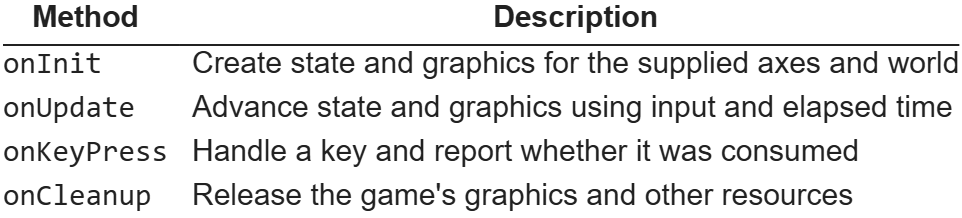
The launcher calls onUpdate on its active game, and MATLAB dispatches that call to the selected subclass. Pong implements paddle and ball movement; Flappy Bird advances its bird and pipes. All games inherit methods for scoring, combo handling and visual effects from GameBase. Window management, menus, timing and common services stay with the launcher.
As a handle class, GameBase lets the launcher keep a reference to the same game instance while its state changes. Position arrays, velocities, scores and graphics handles belong to that instance. Property access attributes allow the host to read the common score while leaving changes under the control of the game classes.
Flappy Bird creates its pipe patches in onInit, then reuses them throughout the game. Their handles and state are stored in private properties of the game instance. Its onUpdate method moves the active pipes across the playfield. Spawning a pipe selects an available pair, assigns its position and gap, and adds it to the active list. Once it leaves the playfield, the pair is hidden and its slot becomes available again:

In the default gravity-and-flap mode, the onKeyPress input handler sets a pending flap flag. The next update applies the upward impulse and clears the flag.
When the window closes, Arcade stops and deletes its timer, calls the active game's onCleanup method and clears its effects before deleting the figure. The smaller examples use MATLAB's onCleanup object to delete their own figure when the function exits. The requestClose callback function assigned to the figure’s CloseRequestFcn property sets a stop flag, letting the current update finish before cleanup removes the graphics.
Recent work on MATLAB graphics and performance
The MathWorks graphics team has also been improving the underlying rendering system. Maddie Moon's article about WebGL describes the R2025a transition, which brought the renderer already used by uifigure to regular MATLAB figures, along with work on stability, consistency and smoothing. Will Jackson also explains related changes to built-in panning, zooming and rotation in his article on the new interactions system.
R2025b focused on quality and stability improvements, building on the changes introduced in R2025a. It also improved performance when capturing successive frames in a loop with getframe, the function used by Arcade’s recording helper to capture and store frames for GIFs and videos.
R2026a included memory and stability improvements for graphics such as scatter and surface plots, described in Adam Danz's overview and the release notes. In addition, Jessa Karlberg describes the redesigned axes toolbar in R2026a, which allows seamless hovering without the animation slowdown issues caused by the toolbar’s continuous mouse tracking in earlier releases, eliminating the need to remove the toolbar as a workaround.
R2026b improved responsiveness for large data visualizations, with plot and plot3 being able to display lines and markers incrementally and shortening the wait time for the first visible results. MathWorks also reports automatic selection of a dedicated rendering GPU on supported Windows and Linux systems with multiple GPUs. These changes are documented in the release notes and the GPU-selection update.
info = rendererinfo;
info.GraphicsRenderer
info.RendererDevice
Mike Croucher also describes a new object-management system for R2026b, which can speed up object-oriented MATLAB code by reducing the cost of creating and deleting objects, as well as accessing their properties. The system is currently available as a beta and can be enabled through a package on File Exchange. Its documentation explains the changes to object lifecycle and compatibility.
Developing MATLAB code with AI
Arcade was developed with Claude Code through the MATLAB MCP Server, and the contest welcomes AI assistance as an option.
When working with an AI assistant, consider sharing your project's requirements and any existing code it can build on. Arcade's developer guide, for example, describes the shared game interface and explains how to add a new game. For your own game, you could begin with the main interaction and add features gradually, playing and improving it as you go. When something goes wrong, describe what happened and how to reproduce the problem, such as a ball passing through a wall at higher speeds.
The MATLAB Agentic Toolkit provides workflows for code review, analysis and testing. Its setup guide covers connecting MATLAB to AI applications including Claude Code, GitHub Copilot, OpenAI Codex, Gemini CLI and Amp, and installing MATLAB-specific skills. Through the MCP server, the AI assistant can run MATLAB code and tests, inspect the results, and use them to help diagnose problems and revise the code.
Several implementation choices in Arcade align with the MATLAB Coding Guidelines and performance rules: using a handle class for an object whose identity persists, restricting access to its state, retaining graphics, preallocating known-size arrays and cleaning up timers. The two downloadable examples presented above were checked with MATLAB Code Analyzer and tested for resizing, input, handle reuse and cleanup.
I hope that this article gives you something to experiment with, and perhaps a starting point for the One-Button Game Mini Hack. I look forward to seeing what you make!

Hi there,
Is there a change in the json response when I do http write to a channel ?
I send:
POST /update.json HTTP/1.1
Content-Type: application/x-www-form-urlencoded
Host: api.thingspeak.com
Connection: close
Content-Length: 102
apikey=xxxxxxxxxxxx&field1=-4.803&field3=18&field4=91&field5=109&field6=56&field7=0&field8=7
and I don't receive the normal response
I get sth like:
'unsafe-eval'; style-src 'self' https: 'unsafe-inline'; connect-src 'self' https: https://*.mathworks.com https://*.thingspeak.com https://*.omtrdc.net https://*.demdex.net; frame-src 'self' https: https://*.mathworks.com

Once you've uploaded your one-button game, it doesn't seem like there's a way to edit/update it. That's led me to fall into a couple of traps. One has a simple solution, so I'll share it. The other has me still scratching my head, so I'll open it up for discussion.
- Restarting. While you're developing and testing in MATLAB, it's easy enough to close the window and rerun your game. But the process is clunkier in the online gallery, so make sure your game includes a clean way to restart. If you're using an agent, it's easy enough to instruct it to modify the spacebar/click callback when the game ends so that it now calls the start/initialization function. This is a nice job for an agent (standard coding pattern it will probably do right, while I'll mess up and get annoyed).
- Timing. I can't figure out how to translate frame rate on my slow desktop MATLAB to the online running framework. Things that seem very sedate while testing suddenly get very exciting when I upload. Anyone know a good way to emulate just how zippy the real game will be?

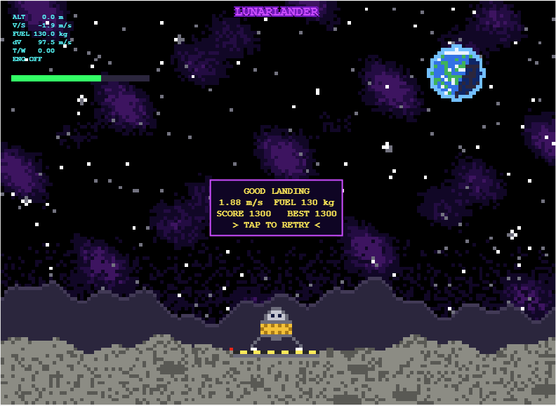
My entry for the one-button game mini hack Lunar Lander - Tap to Burn, is a one-button powered descent. You start 500 m above the surface, falling at 10 m/s, with 200 kg of propellant. One tap turns on the engine, and the next tap stops it.
How scoring works
- Crash: landing at 3 m/s or faster scores 0.
- Abort: rising above 750 m scores 0.
- Safe landing: below 3 m/s scores 10 points per kilogram of fuel remaining.
- Perfect touchdown: below 1 m/s doubles the reward to 20 points per kilogram of fuel remaining.
Physics in the game
- Fuel mass decreases as propellant is burned.
- Gravity continuously accelerates the lander downward.
- The engine does not reach full thrust instantly, so timing matters.
- The display turning red indicates when a full thrust landing burn becomes possible.
Display readouts
- ALT [m]: Height above the surface.
- V/S [m/s]: Vertical speed.
- FUEL [kg]: Remaining propellant.
- dV [m/s]: remaining velocity change the fuel can provide, from the rocket equation Δv=Isp·g₀·ln(m/m_dry).
- T/W: Thrust to weight ratio.
My best so far is 1300. Has anyone managed a sub 1m/s landing?

The day and night colours depend on how far the fox has run. Instead of recolouring everything on every frame, I turn the cycle into a small number of steps and only recolour when the step changes:
nn=.5-.5*cos(2*pi*s.dist/3200);
q=round(nn*40);
if ~isequal(s.ax.UserData,q)
s.ax.UserData=q;
% recolour the background, ground, text and obstacles here
end
The current step is stored in the axes UserData, so the check is cheap. Text works the same way. I only set a text string when the new string is different from the old one:
if ~strcmp(s.sct.String,t), s.sct.String=t; end
Setting properties that have not changed still costs time in every frame, so skipping them helps a lot in a game that redraws many times per second.
Check against your code: the first block is simplified from your renderFrame. Your real code also adds +100*(s.st==2) to q so the colours change on the game-over screen, and I left that out to keep the tip simple. The strcmp line is from your score text. Both matc
The day and night colours depend on how far the fox has run. Instead of recolouring everything on every frame, I turn the cycle into a small number of steps and only recolour when the step changes:
nn=.5-.5*cos(2*pi*s.dist/3200);
q=round(nn*40);
if ~isequal(s.ax.UserData,q)
s.ax.UserData=q;
% recolour the background, ground, text and obstacles here
end
The current step is stored in the axes UserData, so the check is cheap. Text works the same way. I only set a text string when the new string is different from the old one:
if ~strcmp(s.sct.String,t), s.sct.String=t; end
Setting properties that have not changed still costs time in every frame, so skipping them helps a lot in a game that redraws many times per second.
All the graphics objects (patches, lines and text) are created one time, when the game starts. After that, the render function only changes their data with set:
set(s.hd,'XData',s.DS{k}+DX,'YData',s.DT{k}+G+s.dy)
Creating new objects on every frame is a common reason MATLAB games feel slow. Updating objects that already exist is much cheaper. To hide an object, I set its data to NaN instead of deleting it:
set(s.ho(m),'XData',NaN,'YData',NaN)
Disclosure: the game code was written with Claude (an AI assistant). I tested the game in MATLAB and checked the details myself.
For the One-button Game Mini Hack, the code limit is 10,000 characters. I made a game called Ember Fox, where a fox runs and a stone guardian chases it, and you have one button. These are the techniques in the code that I found most useful.
Tip 1: Draw pixel-art sprites from text
Each sprite is stored as a grid of characters, where # is a filled pixel and . is empty:
A=['######';'#.##.#';'######';'.####.'];
[X,Y]=spr(A,0.6);
A helper function, spr, turns the grid into rectangles. For each row it uses diff to find where every run of # starts and ends, and each run becomes one rectangle instead of one rectangle per pixel. This keeps the sprite data small and the number of graphics objects low. All the sprites are built once, when the game starts.

If you are as excited as me to play these games but somehow something is stopping you from doing just that, you are at the right place. Follow the steps below and you will be playing in no time (maybe some time depending on your browser, network speed, etc.):
- Click on the game you like the look of (let's say, something that is transformative).
- This will open up its details page with the game code, preview video and the "Play Game" button. Click the video or the button.
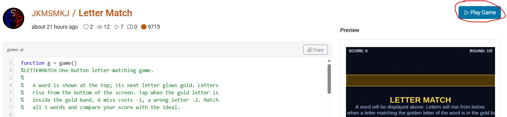
- This will open up "MATLAB Drive" in a new browser window with a preview screenshot of a half-played game and a "Run this App" button. Click this button and nothing will seem to happen at first. And nothing will happen at any other subsequent tries. But don't worry, that's why you're here.
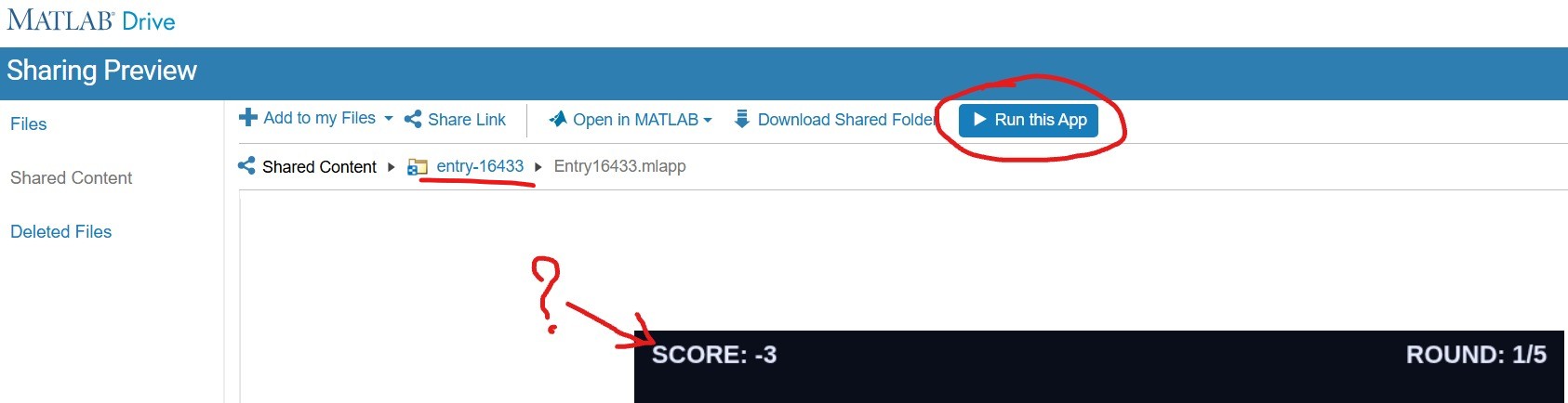
- Click on the "entry-×××××" blue hyperlink just above the preview area (underlined in red above). This will take you to a list of two files but hide the crucial blue button. Click on the "Entry×××××.mlapp" file to resurface the blue button.
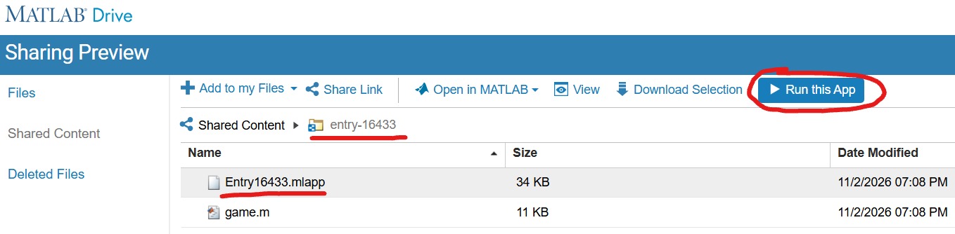
- With expectant hands, click the "Run this App" button. This time it will reload the "MATLAB Drive" and put it in the mode to run your chosen game.
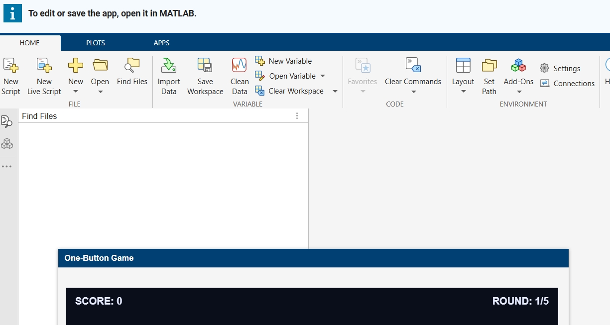
- Finally, you are where you expected to be in the point 3! Enjoy your game.🥳
Hi everyone,
I made Ember Fox: Outrun the Stone Guardian for the One-button Game Mini Hack. A fox runs forward, and a stone guardian rolls behind it and chases it. You must hop over obstacles to stay ahead.
Play it here: https://www.mathworks.com/matlabcentral/communitycontests/contests/10/entries/16448
(Click Play Game, then Run this App.)
The whole game fits in less than 10,000 characters. Below are the main tricks I used. I hope they help you with your own games.
How the game works
- One button does everything: tap to hop, tap again in the air to dive.
- If you hit an obstacle, the stone guardian gets closer. If it catches you, the game ends.
- Diving onto a flying enemy gives bonus points.
- Power-ups give a shield, slow motion, or push the guardian back.
- Passing obstacles builds a combo multiplier.
- The game gets faster the longer you play, and the sky changes from day to night.
Trick 1: Draw pixel-art sprites from text
I draw each sprite as a grid of characters. A # means a filled pixel:
A=['######';'#.##.#';'######';'.####.'];
[X,Y]=spr(A,0.6);
My helper function spr turns each row into rectangles. It uses diff to find where every run of # starts and ends. One run becomes one rectangle, not one rectangle per pixel. This keeps the number of graphics objects low and the code short.
Trick 2: Create graphics once, then only update them
In init I create every patch, line and text object one time. In renderFrame I only change them with set:
set(s.hd,'XData',s.DS{k}+DX,'YData',s.DT{k}+G+s.dy)
Creating new objects every frame makes a game slow. Updating existing ones is much faster. To hide an object, I set its data to NaN instead of deleting it.
Trick 3: Update only what changed
The day and night colours depend on how far you have run. I turn the cycle into a small number of steps and change the colours only when the step changes:
nn=.5-.5*cos(2*pi*s.dist/3200);
q=round(nn*40);
if ~isequal(s.ax.UserData,q)
s.ax.UserData=q; % change all colours here
end
I do the same for text. I only set the text when the new text is different:
if ~strcmp(h.String,t), h.String=t; end
Trick 4: One button, different actions
The game state decides what the button does:
- On the start or game-over screen, it starts the game.
- On the ground, it makes the fox hop.
- In the air, it makes the fox dive down faster.
This gives the player more choices without adding more buttons.
Trick 5: Smooth difficulty and simple collisions
The speed grows quickly at first, then slows down, so the game stays fair:
s.spd=55+90*(1-exp(-s.sc/900));
Collisions are simple rectangle checks. After a hit, the fox is safe for a short time, so one mistake does not cause many hits in a row.
Trick 6: Fit the character limit
- Use short variable names.
- Use loops and shared code instead of repeating lines.
- Run minihackContest.validate often to check the character count.
Known problem: the game runs smoothly in desktop MATLAB, but it can lag in MATLAB Online. For the best experience, run it on your computer with minihackContest.play.
Thank you for reading! If you have questions or ideas to make it better, please write a comment. I would love to see how you solve these problems in your own games.

I have MATLAB R2026b, the MATLAB Agentic Toolkit, and Claude Code installed.
In the first session, I asked Claude (Opus 5.5, High effort) to review the game rules, suggest MATLAB Agentic Toolkit skills, install them inside the project folder, and create a CLAUDE.md file.
In the second session, I asked Claude to create a combat game in which the player controls a simple stick figure wielding a club; clicking makes the figure swing the club. Simple monsters approach the player and drain the player’s health on contact, while hitting a monster with the club eliminates it. The game has an old-school 2D look, with a dark blue, star-filled background and light blue characters.
That's it. You can see result here: CLUB NIGHT
My best score until now is 2060.
Let me know your best score in the comments.


I started my game for this contest, Stack OverDad, one month before the contest began. Dad tells programming jokes at the dinner table, and you have to laugh at the right moment. I was very happy with it. It had a dog, a little brother with a spoon, a window with a sun that goes down, fifty jokes, and many small animations.
Then the contest started, and I read the rules again. One line said: each entry is limited to 10,000 characters of MATLAB code.
My code had more than 70,000 characters.
So, as you can guess, the next hourse were cut, test, cut, test, cut... In this post, I will tell you what I learned on the way (from my AI friend!). Some of it surprised me.
Step 1: Cut What the Player Does Not Feel
For every part of the game, I asked: "Does the player really feel this?"
The dog: cute, but no. The brother: funny, but no. The sunset: nobody looks at the window when Dad tells a joke. Forty jokes: a game only uses ten anyway.
This was the biggest step, and the hardest, because I liked all of these things. But the game did not get worse. It got clearer. After this, my file had about 9,800 characters. I was done!
Step 2: The Surprise
The contest project has a command to check the game before you submit it:
minihackContest.validate
I ran it, and it said:
Validation failed: game.m exceeds the character limit (16145 / 10000, comments excluded).
16,145? My file had 9,800 characters. I counted again. It still had 9,800.
So I opened the validator to see how it counts. This is the line:
charCount = strlength(char(tree2str(mtree(gameFile, '-file'))));
mtree reads the code into a tree, and this removes the comments. Then tree2str writes the code again, in a clean, standard layout. The validator counts that text, not my file.
And the clean layout is not short at all. For example, this one line of mine:
if p,pr(s.T);end
comes back from tree2str like this:
if p
pr( s.T );
end
Every statement gets its own line. Every line gets indentation. Every f(a,b) becomes f( a, b ), and every [1 2 3] becomes [ 1, 2, 3 ]. My short style was not short anymore.
The good news: now I knew the real rule, so I could play by it.
Step 3: What Is Cheap and What Is Expensive
- Expensive: many statements, deep nesting, and long lists of numbers.
- Cheap: text inside a string. tree2str does not change a string at all.
So the plan was: fewer statements, less nesting, and move numbers into strings.
Example 1: Many Values in One Statement
s.st = 3;
s.t0 = t;
s.la = -1;
becomes one statement with deal:
[s.st, s.t0, s.la] = deal(3, t, -1);
Example 2: A Small if Without if
if n == 1
s.fl = "TEN?!";
end
With logical indexing, it is one line. If the condition is false, nothing changes:
s.fl(n == 1) = "TEN?!";
Example 3: Many Strings in One String
A list like ["PERFECT!", "GOOD!", "TOO LATE..."] pays for every ", ". One string with a separator is cheaper:
B = split("PERFECT!|GOOD!|TOO LATE...", "|");
All fifteen jokes are now one string too.
Example 4: Numbers Inside a String
This was the biggest trick. My scene (the table, the chairs, Dad, the family) is made of rectangles, ellipses, and polygons. That is hundreds of numbers.
So I stored each number as one character in a string. A character is really a number (its code), so I can turn it back:
v = double(char(z))/20 - 1025; % every character of z becomes one number again
I chose codes from a big block of normal, printable characters. They look like Chinese characters, but they are not words. I only use their codes. One small loop reads the string and draws all the shapes with patch. Now the whole scene costs about one character per number.
One warning from my own mistake: use double(char(z)), not double(z). If z is a string, double(z) gives NaN. My first test showed an empty table because of this.
I kept the readable list of shapes in a separate file, and it writes the packed strings for me.
I Had Help
I worked with an AI assistant the whole way. It read the validator with me, tested many small ideas fast, measured which part of the code cost the most, and rewrote code again and again without getting tired.
But the AI did not decide what the game is. It could tell me that the dog costs 1,700 characters. It could not tell me if the dog is worth it. Every "keep" or "cut" was my choice. I think this is the best way to work with AI: let it do the heavy lifting, and keep the decisions for yourself.
The Result
The validator now says 9,936 characters. The game still has Dad, THE LOOK, Mom's warnings, the family walking out, the ranks, and fifteen jokes.
My advice: run minihackContest.validate early. Do not count the characters yourself, because the validator does not count your file. It counts the clean version of your file.
I hope you have found this helpful. Thank you for reading.

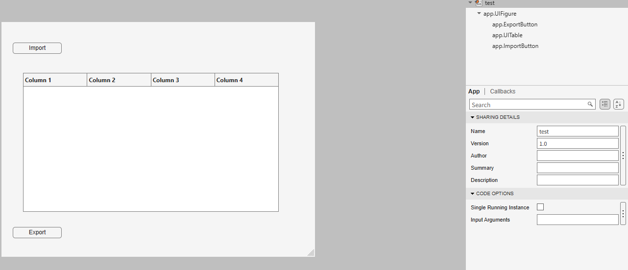
Hello everyone, I am new to Matlab.
I am trying to create an app to export the 5th column into a new sheet in the imported Excel file when I click Export button.
How can I write code in ExportButtonPushed
classdef test < matlab.apps.AppBase
% Properties that correspond to app components
properties (Access = public)
UIFigure matlab.ui.Figure
ExportButton matlab.ui.control.Button
UITable matlab.ui.control.Table
ImportButton matlab.ui.control.Button
end
% Callbacks that handle component events
methods (Access = private)
% Button pushed function: ImportButton
function ImportButtonPushed(app, event)
[file, location] = uigetfile( ...
{'*.xlsx;*.xlsm', 'Excel files'; '*.txt', 'Text files'; '*.*', 'All files'}, ...
'File Selector');
figure(app.UIFigure)
if isequal(file, 0), return, end
fullPath = fullfile(location, file);
try
[~,~,ext] = fileparts(fullPath);
if any(strcmpi(ext, {'.xlsx','.xlsm','.xls'}))
T = readtable(fullPath, 'Sheet', 1, 'VariableNamingRule', 'preserve');
else
T = readtable(fullPath, 'VariableNamingRule', 'preserve');
end
catch ME
uialert(app.UIFigure, ME.message, 'Read error');
return
end
if width(T) < 5
uialert(app.UIFigure, 'The file needs at least 5 columns.', 'Import error');
return
end
app.UITable.Data = T;
app.UITable.ColumnName = T.Properties.VariableNames;
lengthlist = T{:,5};
end
% Button pushed function: ExportButton
function ExportButtonPushed(app, event)

Recently, I encountered an issue where solve returned no solution for a system of equations, even though the system obviously has solutions. This can be easy to overlook.
For example:
syms a b c x
equs = [a*x^2+b*x+c==0;
a==1];
St = solve(equs,x)
St is returned as an empty set, suggesting that there is no solution???
However, since a is constrained by the equation a == 1, the correct way is:
S = solve(equs,[x,a])
disp(S.x)
disp(S.a)
Here, a must also be included in the list of variables to solve for. Only then will solve treat a as an unknown, apply the constraint a == 1, and substitute it into the equation during the solving process.
symvar(equs)
Based on the output of the symvar function, a is already identified as one of the symbolic variables (unknowns) in the system of equations. However, the actual behavior of solve appears to contradict this expectation. In practice, a must still be explicitly included in the variable list passed to solve; otherwise, it is treated as a symbolic parameter rather than a variable to be solved for.
Takeaway: When using solve for a system of equations, any symbol that appears in the equations and is constrained by additional equations (such as a == 1) should generally be included in the variable list. Otherwise, solve may treat it as a symbolic parameter rather than an unknown, which can lead to an empty solution set or unexpected results.
Am I missing something here? I'd love to hear your thoughts.

As a long-standing request from users, we are happy to announce that HDFql now supports MATLAB for managing HDF5 and MAT files.
In short, HDFql (Hierarchical Data Formal query language) is the first high-level, declarative language for managing HDF5 or MAT data. Designed to be as simple and powerful as SQL, it dramatically reduces the learning effort and time required to work with HDF5. With its intuitive syntax, HDFql provides a clean interface for reading and writing HDF5 data across programming languages (C, C++, Java, Python, C#, Fortran, R, and now MATLAB) and platforms (Windows, Linux, and macOS). In addition, HDFql is based on a flexible parallel architecture that transparently leverages available cores and, in MPI clusters, nodes to efficiently process large volumes of data.
Key benefits of HDFql include enabling users to replace dozens of lines of complex HDF5 code with just a few lines of simple code, helping AI models generate better code using far fewer tokens, and making AI-generated code easier for humans to review.
Happy coding, prompting, or reviewing with HDFql in MATLAB!

We use Timecontrol for statistic automations. Yesterday at 2026-10-220 10:00pm CET Time control stopped working. There is new new time in the "Run At" field, although the script should run every 5 minutes. We had the same problem in September, see https://de.mathworks.com/matlabcentral/answers/2184870-thingspeak-timecontrol-stopped-working-at-all?s_tid=srchtitle
Has anybody also prolems with Timecontrol?

I am frequently facing issue with the onramp training of not proceeding to the next task or section, even after successfully completion of the current task or complete section.

For the past several days I have been experiencing a problem with data visualization on two of my ThingSpeak channels.
The data appears to be uploaded and stored correctly, and new entries are still being added to the channels. However, the visualizations are not working correctly.
The standard Field Charts show only a very small number of data points instead of the normal continuous measurements. Most of the points are compressed on the left side of the chart, while one or a few points appear far to the right and are connected by long straight lines. The time axis is also incorrect and sometimes shows repeated dates such as “01 Jan”.
The numeric widgets are affected as well and display incorrect values. Some custom visualizations also remain blank or fail to load.
The problem appeared suddenly and affects two separate channels which had previously been working correctly. I did not make any significant changes to the channels before the problem started.
This seems somewhat similar to the ThingSpeak chart/timeline issue reported in June 2026, when charts were displaying incorrect time ranges and the DAYS/RESULTS settings were not working correctly. However, my current problem also affects numeric widgets and custom visualizations, and the charts show incorrect dates and strangely positioned data points.
Could this be a regression or a similar issue with the ThingSpeak visualization system?
Has anyone else experienced the same problem recently?

The Ran In tag still shows R2026a on Answers and Discussions (as does the Executing In popup), even though both are actually running R2026b.
This seems to be always be an issue whenver the site updates to the latest release. Seems like it should be pretty straightforward to update those message at the same time the underlying release is updated. Or am I underestimating the complexity of that task?
matlabRelease

What if MATLAB could show you not only the final output, but also how your code reaches that result?
Imagine an interactive tool that visualizes variable changes, function calls, matrix transformations, and execution flow as a program runs. Engineers could watch algorithms evolve, identify unexpected behavior, and understand complex simulations through live visualizations.
The idea is to build a Live MATLAB Execution Explorer that combines code tracing, variable timelines, and 3D engineering simulations in one interface.
From debugging control systems to teaching numerical methods, this could transform how students, researchers, and engineers interact with code.
The challenge? Capturing execution data efficiently without significantly affecting performance.
The vision: Turn programming from something we read into something we can see, explore, and understand.
#MATLAB #Simulink #EngineeringInnovation #Simulation #DeveloperTools

I recently had an idea for a side project: building an app/extension that can interactively follow simulations and visualise the live flow of code execution.
For this, I would need access to variables, datasets, and the function call stack during execution, ideally without interfering with the actual code execution.
However, I found that MATLAB's current architecture makes this difficult, as the entire application runs in a single thread and there are no publicly exposed APIs to access runtime variables without interrupting execution.
Can anyone suggest a possible workaround or an alternative approach to achieve this?

