Raised Cosine Filtering
This example shows the intersymbol interference (ISI) rejection capability of the raised cosine filter, and how to split the raised cosine filtering between transmitter and receiver, using raised cosine transmit and receive filter System objects.
Raised Cosine Filter Specifications
The main parameter of a raised cosine filter is its roll-off factor, which indirectly specifies the bandwidth of the filter. Ideal raised cosine filters have an infinite number of taps. Therefore, practical raised cosine filters are windowed. The window length is controlled using the FilterSpanInSymbols property. In this example, you specify the window length as six symbol durations because the filter spans six symbol durations. Such a filter also has a group delay of three symbol durations. Raised cosine filters are used for pulse shaping, where the signal is upsampled. Therefore, you also need to specify the upsampling factor. These parameters are used to design the raised cosine filter for this example.
% Define the parameters
Nsym = 6;                                 % Filter span in symbol durations
beta = [0.1, 0.3, 0.5, 0.7, 0.9];         % Roll-off factor
sampsPerSym = 8;                          % Upsampling factor
colors = ["r", "g", "b", "c", "m"];       % Define colors for different beta values
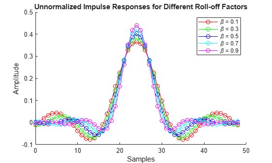
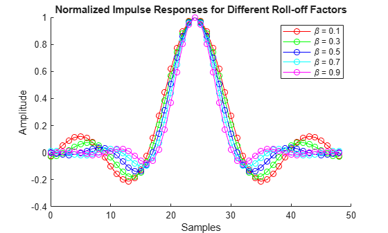
Create a raised cosine transmit filter System object™ for each beta value and set its properties to obtain the desired filter characteristics. Use impz to visualize filter characteristics. The raised cosine transmit filter System object designs a direct-form polyphase FIR filter with unit energy. The filter has an order of Nsym*sampsPerSym, or Nsym*sampsPerSym+1 taps. You can utilize the Gain property to normalize the filter coefficients so that the filtered and unfiltered data matches when overlayed.
% Create figures for plotting
figure(Name="Unnormalized Impulse Responses");
hold on;
figure(Name="Normalized Impulse Responses");
hold on;

for i = 1:length(beta)
    % Create a raised cosine transmit filter for each beta value
    rctFilt = comm.RaisedCosineTransmitFilter(RolloffFactor=beta(i), ...
        FilterSpanInSymbols=Nsym, ...
        OutputSamplesPerSymbol=sampsPerSym);

    % Extract the filter coefficients
    b = coeffs(rctFilt);

    % Compute the unnormalized impulse response
    [h_unnorm, t_unnorm] = impz(b.Numerator);

    % Switch to the unnormalized figure to plot
    figure(findobj(Name="Unnormalized Impulse Responses"));
    plot(t_unnorm, h_unnorm, colors(i), Marker="o", ...
        DisplayName=['\beta = ', num2str(beta(i))]);

    % Normalize the filter coefficients
    rctFilt.Gain = 1/max(b.Numerator);

    % Compute the normalized impulse response
    [h_norm, t_norm] = impz(b.Numerator * rctFilt.Gain);

    % Switch to the normalized figure to plot
    figure(findobj(Name="Normalized Impulse Responses"));
    plot(t_norm, h_norm, colors(i), Marker="o", ...
        DisplayName=['\beta = ', num2str(beta(i))]);
end

% The unnormalized figure
figure(findobj(Name="Unnormalized Impulse Responses"));
hold off;
title("Unnormalized Impulse Responses for Different Roll-off Factors");
xlabel("Samples");
ylabel("Amplitude");
legend("show");
figure(findobj('Name', 'Normalized Impulse Responses'));
hold off;
title("Normalized Impulse Responses for Different Roll-off Factors");
xlabel("Samples");
ylabel("Amplitude");
legend show;
Pulse Shaping with Raised Cosine Filters
Generate a bipolar data sequence, and use the raised cosine filter to shape the waveform without introducing ISI.
% Parameters
DataL = 20;             % Data length in symbols
R = 1000;               % Data rate
Fs = R * sampsPerSym;   % Sampling frequency

% Create a local random stream to be used by random number generators for
% repeatability
hStr = RandStream('mt19937ar',Seed=0);

% Generate random data
x = 2*randi(hStr,[0 1],DataL,1)-1;
% Time vector sampled at symbol rate in milliseconds
tx = 1000 * (0: DataL - 1) / R;
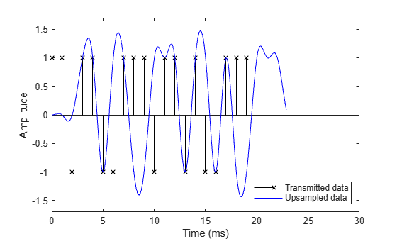
Compare the digital data and the interpolated signal in a plot. It is difficult to compare the two signals because the peak response of the filter is delayed by the group delay of the filter (Nsym/(2*R)). Append Nsym/2 zeros at the end of input x to flush all the useful samples out of the filter.
% Design raised cosine filter with given order in symbols
rctFilt1 = comm.RaisedCosineTransmitFilter(...
  Shape='Normal', ...
  RolloffFactor=0.5, ...
  FilterSpanInSymbols=Nsym, ...
  OutputSamplesPerSymbol=sampsPerSym);


% Normalize to obtain maximum filter tap value of 1
b1 = coeffs(rctFilt1);
rctFilt1.Gain = 1/max(b1.Numerator);

% Visualize the impulse response
%impz(rctFilt.coeffs.Numerator)

% Filter
yo = rctFilt1([x; zeros(Nsym/2,1)]);
% Time vector sampled at sampling frequency in milliseconds
to = 1000 * (0: (DataL+Nsym/2)*sampsPerSym - 1) / Fs;
% Plot data
fig1 = figure;
stem(tx, x, 'kx'); hold on;
% Plot filtered data
plot(to, yo, 'b-'); hold off;
% Set axes and labels
axis([0 30 -1.7 1.7]);  xlabel('Time (ms)'); ylabel('Amplitude');
legend('Transmitted data','Upsampled data','Location','southeast')
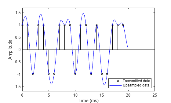
Compensate for the raised cosine filter group delay by delaying the input signal. Now it is easy to see how the raised cosine filter upsamples and filters the signal. The filtered signal is identical to the delayed input signal at the input sample times. This result shows the raised cosine filter capability to band-limit the signal while avoiding ISI.
% Filter group delay, since raised cosine filter is linear phase and
% symmetric.
fltDelay = Nsym / (2*R);
% Correct for propagation delay by removing filter transients
yo = yo(fltDelay*Fs+1:end);
to = 1000 * (0: DataL*sampsPerSym - 1) / Fs;
% Plot data.
stem(tx, x, 'kx'); hold on;
% Plot filtered data.
plot(to, yo, 'b-'); hold off;
% Set axes and labels.
axis([0 25 -1.7 1.7]);  xlabel('Time (ms)'); ylabel('Amplitude');
legend('Transmitted data','Upsampled data','Location','southeast')
Roll-off Factor
Show the effect that changing the roll-off factor from .5 (blue curve) to .2 (red curve) has on the resulting filtered output. The lower value for roll-off causes the filter to have a narrower transition band causing the filtered signal overshoot to be greater for the red curve than for the blue curve.
% Set roll-off factor to 0.2
rctFilt2 = comm.RaisedCosineTransmitFilter(...
  Shape='Normal', ...
  RolloffFactor=0.2, ...
  FilterSpanInSymbols=Nsym, ...
  OutputSamplesPerSymbol=sampsPerSym);
% Normalize filter
b = coeffs(rctFilt2);
rctFilt2.Gain = 1/max(b.Numerator);
% Filter
yo1 = rctFilt2([x; zeros(Nsym/2,1)]);
% Correct for propagation delay by removing filter transients
yo1 = yo1(fltDelay*Fs+1:end);
% Plot data
stem(tx, x, 'kx'); hold on;
% Plot filtered data
plot(to, yo, 'b-',to, yo1, 'r-'); hold off;
% Set axes and labels
axis([0 25 -2 2]);  xlabel('Time (ms)'); ylabel('Amplitude');
legend('Transmitted Data','beta = 0.5','beta = 0.2', ...
    'Location','southeast')

Square-Root Raised Cosine Filters
A typical use of raised cosine filtering is to split the filtering between transmitter and receiver. Both transmitter and receiver employ square-root raised cosine filters. The combination of transmitter and receiver filters is a raised cosine filter, which results in minimum ISI. Specify a square-root raised cosine filter by setting the shape as 'Square root'.
% Design raised cosine filter with given order in symbols
rctFilt3 = comm.RaisedCosineTransmitFilter(...
  Shape="Square root", ...
  RolloffFactor=0.5, ...
  FilterSpanInSymbols=Nsym, ...
  OutputSamplesPerSymbol=sampsPerSym);
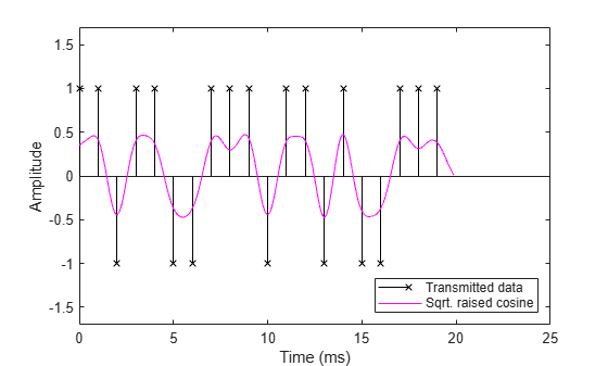
Upsample and filter the data at the transmitter using the designed filter. This plot shows the transmitted signal when filtered using the square-root raised cosine filter.
% Upsample and filter.
yc = rctFilt3([x; zeros(Nsym/2,1)]);
% Correct for propagation delay by removing filter transients
yc = yc(fltDelay*Fs+1:end);
% Plot data.
stem(tx, x, 'kx'); hold on;
% Plot filtered data.
plot(to, yc, 'm-'); hold off;
% Set axes and labels.
axis([0 25 -1.7 1.7]);  xlabel('Time (ms)'); ylabel('Amplitude');
legend('Transmitted data','Sqrt. raised cosine','Location','southeast')
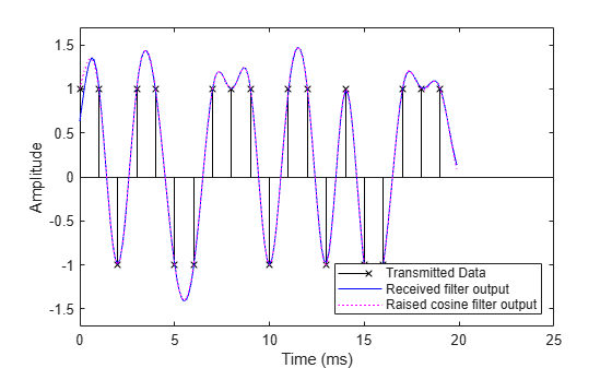
Then, filter the transmitted signal (magenta curve) at the receiver (Do not decimate the filter output to show the full waveform). The default unit energy normalization ensures that the gain of the combination of the transmit and receive filters is the same as the gain of a normalized raised cosine filter. The filtered received signal, which is virtually identical to the signal filtered using a single raised cosine filter, is depicted by the blue curve at the receiver.
% Design and normalize filter.
rcrFilt = comm.RaisedCosineReceiveFilter(...
  'Shape',                  'Square root', ...
  'RolloffFactor',          0.5, ...
  'FilterSpanInSymbols',    Nsym, ...
  'InputSamplesPerSymbol',  sampsPerSym, ...
  'DecimationFactor',       1);
% Filter at the receiver.
yr = rcrFilt([yc; zeros(Nsym*sampsPerSym/2, 1)]);
% Correct for propagation delay by removing filter transients
yr = yr(fltDelay*Fs+1:end);
% Plot data.
stem(tx, x, 'kx'); hold on;
% Plot filtered data.
plot(to, yr, 'b-',to, yo, 'm:'); hold off;
% Set axes and labels.
axis([0 25 -1.7 1.7]);  xlabel('Time (ms)'); ylabel('Amplitude');
legend('Transmitted Data','Received filter output', ...
    'Raised cosine filter output','Location','southeast')
Impact of Rolloff Factor on PAPR for Single Carrier Systems
Peak-to-average power ratio (PAPR) is a measure that quantifies how extreme the peaks of a signal can be compared to its average power level. A high PAPR indicates that, at times, the signal has very high peak values relative to its average power, which is challenging for power amplifiers and leads to nonlinear distortion.
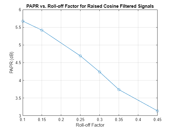
The roll-off factor in a raised cosine filter determines the transition bandwidth of the filter from its passband to stopband. A lower roll-off factor means a sharper transition, which leads to more efficient bandwidth usage but potentially higher PAPR. The sharper transitions in the frequency domain can lead to higher peak amplitudes in the time domain.
Conversely, a higher roll-off factor results in a smoother transition in the frequency domain, which leads to a lower PAPR because the signal's time-domain peaks are less pronounced. However, this result comes at the cost of increased bandwidth usage.
This example demonstrates the effect of the roll-off factor on the PAPR of binary phase shift keying (BSPK) signal in a single carrier system.
N = 10000; % Number of bits
M = 2;     % Modulation order (BPSK in this case)
rolloffFactors = [0.1, 0.15, 0.25, 0.3, 0.35, 0.45];
sampsPerSym = 2;
Nsym = 6;  % Filter span in symbols

% Generate a random binary signal
data = randi([0 M-1], N, 1);

% BPSK Modulation
modData = pskmod(data, M);

% Initialize vector to store PAPR values
paprValues = zeros(length(rolloffFactors), 1);

for i = 1:length(rolloffFactors)
    % Create raised cosine transmit filter
    rctFilt = comm.RaisedCosineTransmitFilter(...
        RolloffFactor=rolloffFactors(i), ...
        FilterSpanInSymbols=Nsym, ...
        OutputSamplesPerSymbol=sampsPerSym);
    % Filter the modulated data
    txSig = rctFilt(modData);
    % Create a powermeter object for PAPR measurement
    meter = powermeter(Measurement="Peak-to-average power ratio", ...
        ComputeCCDF=true);
    % Calculate PAPR
    papr = meter(txSig);
    paprValues(i) = papr;
end

% Plot PAPR vs. roll-off factor
figure;
plot(rolloffFactors, paprValues, '-o');
xlabel("Roll-off Factor");
ylabel("PAPR (dB)");
title("PAPR vs. Roll-off Factor for Raised Cosine Filtered Signals");
grid on;
Computational Cost
This table compares the computational cost of a polyphase FIR interpolation filter and polyphase FIR decimation filter.
C1 = cost(rctFilt3);
C2 = cost(rcrFilt);
------------------------------------------------------------------------
                    Implementation Cost Comparison
------------------------------------------------------------------------
                        Multipliers  Adders  Mult/Symbol  Add/Symbol
Multirate Interpolator      49         41          49         41
Multirate Decimator         49         48           6.125      6