Specify Toolbox Settings for Linear Analysis Plots
You can configure linear analysis plot settings that persist between MATLAB® sessions.
To open the setting dialog box, at the MATLAB command line, enter the following command.
ctrlpref

In the Linear System Analyzer app, you can also open the settings dialog box by selecting File > Toolbox Preferences.
Units Settings
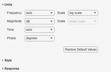
In the Units section configure settings for the following:
Frequency
The default
autooption usesrad/TimeUnitas the frequency units relative to the system time units, whereTimeUnitis the system time units specified in theTimeUnitproperty of the system on frequency-domain plots. For multiple systems with different time units, the units of the first system is used.For the frequency axis, you can select logarithmic or linear scales.
You can also manually select the following frequency units:
Hzrad/srpmkHzMHzGHzrad/nanosecondrad/microsecondrad/millisecondrad/minuterad/hourrad/dayrad/weekrad/monthrad/yearcycles/nanosecondcycles/microsecondcycles/millisecondcycles/hourcycles/daycycles/weekcycles/monthcycles/year
Magnitude
dB— Decibelsabsolute value— Absolute value, which you can plot on a linear or logarithmic scale
Phase — Degrees or radians
Time
The default
autooption uses the time units specified in theTimeUnitproperty of the system on the time- and frequency-domain plots. For multiple systems with different time units, the units of the first system are used.You can also manually select the following time units:
nanosecondsmicrosecondsmillisecondssecondsminuteshoursdaysweeksmonthsyears
Style Settings
In the Style section, you can toggle grid visibility and configure font settings and axes foreground colors for all plots you create.

You have the following choices:
Grids — Activate grids by default in new plots.
Fonts — Set the font size, weight (bold), and angle (italic). Select font sizes from the menus or type any font-size values in the fields.
Colors — Specify the color vector to use for the axes foreground, which includes the X-Y axes, grid lines, and tick labels. Use a three-element vector to represent red, green, and blue (RGB) values. Vector element values can range from 0 to 1.
If you do not want to specify RGB values numerically, click Select to open the Color dialog box.
Response Settings
The Response section has selections for time responses and frequency responses.

For time response plots, the following options are available:
Show settling time within xx% — Set the threshold of the settling time calculation to any percentage from 0 to 100%. The default is 2%.
Specify rise time from xx% to yy% — The standard definition of rise time is the time it takes the signal to go from 10% to 90% of the final value. Specify any percentages you like (from 0% to 100%), provided that the first value is smaller than the second.
For frequency response plots, the following options are available:
Only show magnitude above — Specify a lower limit for magnitude values in response plots so that you can focus on a region of interest.
Wrap phase at — Wrap the phase into the interval [–180º,180º). To wrap accumulated phase across a different interval, enter the lower limit of the interval in the text box. For example, entering 0 causes the plot to wrap the phase into the interval [0º,360º).
Control System Designer Settings
To configure settings for the Control System Designer app, in the Settings dialog box, click Control System Designer.

You can configure the following settings:
Compensator Format — Select the time constant, natural frequency, or zero/pole/gain format. The time constant format is a factorization of the compensator transfer function of the form
where K is compensator DC gain, Tz1, Tz2, ..., are the zero time constants, and Tp1, Tp2, ..., are the pole time constants.
The natural frequency format is
where K is compensator DC gain, ωz1, and ωz2, ... and ωp1, ωp2, ..., are the natural frequencies of the zeros and poles, respectively.
The zero/pole/gain format is
where K is the overall compensator gain, and z1, z2, ... and p1, p2, ..., are the zero and pole locations, respectively.
Bode Options — By default, Control System Designer shows the plant and sensor poles and zeros as blue x's and o's, respectively. Clear this option to eliminate the plant poles and zeros from the Bode plot. The compensator poles and zeros (in red) will still appear.