Prototype and Verify Deep Learning Networks Without Target Hardware
Rapidly prototype your custom deep learning network and bitstream by visualizing intermediate layer activation results and verifying prediction accuracy without target hardware by emulating the network and bitstream. To emulate the network and bitstream, create a dlhdl.Simulator object. Use the dlhdl.Simulator object to:
Retrieve intermediate layer results by using the
activationsfunction.Verify prediction accuracy by using the
predictfunction.
In this example, retrieve the intermediate layer activation results and verify the prediction accuracy for the ResNet-18 network and deep learning processor configuration for the zcu102_single bitstream.
Prerequisites
Deep Learning Toolbox™
Deep Learning HDL Toolbox™
Deep Learning Toolbox Model for ResNet-18 Network
Deep Learning HDL Toolbox Support Package for Xilinx FPGA and SoC Devices
Image Processing Toolbox™
MATLAB® Coder™ Interface for Deep learning
Load Pretrained SeriesNetwork
To load the pretrained network ResNet-18, enter:
snet = resnet18;
To view the layers of the pretrained network, enter:
analyzeNetwork(snet);
The first layer, the image input layer, requires input images of size 224-by-224-by-3, where 3 is the number of color channels.
inputSize = snet.Layers(1).InputSize;
Define Training and Validation Data Sets
This example uses the MathWorks® MerchData data set. This is a small data set containing 75 images of MathWorks merchandise, belonging to five different classes (cap, cube, playing cards, screwdriver, and torch).
curDir = pwd;
unzip('MerchData.zip');
imds = imageDatastore('MerchData', ...
'IncludeSubfolders',true, ...
'LabelSource','foldernames');
[imdsTrain,imdsValidation] = splitEachLabel(imds,0.7,'randomized');
Replace Final Layers
The fully connected layer and the classification layer of the pretrained network net are configured for 1000 classes. These two layers fc1000 and ClassificationLayer_predictions in ResNet-18 contain information on how to combine the features that the network extracts into class probabilities and predicted labels. These layers must be fine-tuned for the new classification problem. Extract all the layers, except the last two layers, from the pretrained network.
lgraph = layerGraph(snet)
lgraph =
  LayerGraph with properties:

     InputNames: {'data'}
    OutputNames: {'ClassificationLayer_predictions'}
         Layers: [71×1 nnet.cnn.layer.Layer]
    Connections: [78×2 table]
numClasses = numel(categories(imdsTrain.Labels))
numClasses = 5
newLearnableLayer = fullyConnectedLayer(numClasses, ...
'Name','new_fc', ...
'WeightLearnRateFactor',10, ...
'BiasLearnRateFactor',10);
lgraph = replaceLayer(lgraph,'fc1000',newLearnableLayer);
newClassLayer = classificationLayer('Name','new_classoutput');
lgraph = replaceLayer(lgraph,'ClassificationLayer_predictions',newClassLayer);
Train Network
The network requires input images of size 224-by-224-by-3, but the images in the image datastores have different sizes. Use an augmented image datastore to automatically resize the training images. Specify additional augmentation operations to perform on the training images, such as randomly flipping the training images along the vertical axis and randomly translating them up to 30 pixels horizontally and vertically. Data augmentation helps prevent the network from overfitting and memorizing the exact details of the training images.
pixelRange = [-30 30];
imageAugmenter = imageDataAugmenter( ...
'RandXReflection',true, ...
'RandXTranslation',pixelRange, ...
'RandYTranslation',pixelRange);
To automatically resize the validation images without performing further data augmentation, use an augmented image datastore without specifying any additional preprocessing operations.
augimdsTrain = augmentedImageDatastore(inputSize(1:2),imdsTrain, ...
'DataAugmentation',imageAugmenter);
augimdsValidation = augmentedImageDatastore(inputSize(1:2),imdsValidation);
Specify the training options. For transfer learning, keep the features from the early layers of the pretrained network (the transferred layer weights). To slow down learning in the transferred layers, set the initial learning rate to a small value. Specify the mini-batch size and validation data. The software validates the network for every ValidationFrequency iteration during training.
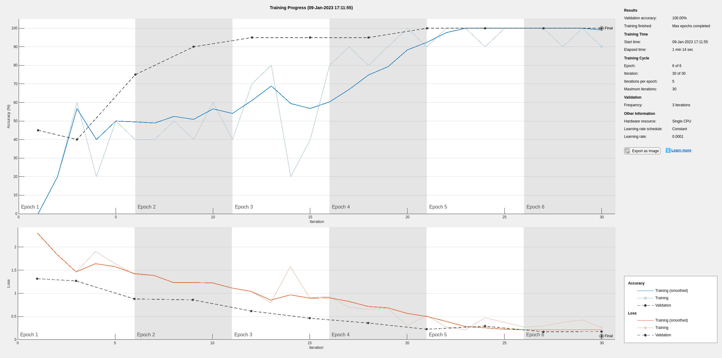
options = trainingOptions('sgdm', ...
'MiniBatchSize',10, ...
'MaxEpochs',6, ...
'InitialLearnRate',1e-4, ...
'Shuffle','every-epoch', ...
'ValidationData',augimdsValidation, ...
'ValidationFrequency',3, ...
'Verbose',false, ...
'Plots','training-progress');
Train the network that consists of the transferred and new layers. By default, trainNetwork uses a GPU if one is available (requires Parallel Computing Toolbox™ and a supported GPU device. See GPU Computing Requirements (Parallel Computing Toolbox)). Otherwise, the network uses a CPU (requires MATLAB Coder Interface for Deep learning). You can also specify the execution environment by using the 'ExecutionEnvironment' name-value argument of trainingOptions.
netTransfer = trainNetwork(augimdsTrain,lgraph,options);
Retrieve Deep Learning Processor Configuration
Use the dlhdl.ProcessorConfig object to retrieve the deep learning processor configuration for the zcu102_single bitstream.
hPC = dlhdl.ProcessorConfig('Bitstream','zcu102_single');
Create Simulator Object
Create a dlhdl.Simulator object with ResNet-18 as the network and hPC as the ProcessorConfig object.
simObj = dlhdl.Simulator('Network',netTransfer,'ProcessorConfig',hPC);
### Optimizing network: Fused 'nnet.cnn.layer.BatchNormalizationLayer' into 'nnet.cnn.layer.Convolution2DLayer'
Compiling leg: conv1>>pool1 ...
Compiling leg: conv1>>pool1 ... complete.
Compiling leg: res2a_branch2a>>res2a_branch2b ...
Compiling leg: res2a_branch2a>>res2a_branch2b ... complete.
Compiling leg: res2b_branch2a>>res2b_branch2b ...
Compiling leg: res2b_branch2a>>res2b_branch2b ... complete.
Compiling leg: res3a_branch1 ...
Compiling leg: res3a_branch1 ... complete.
Compiling leg: res3a_branch2a>>res3a_branch2b ...
Compiling leg: res3a_branch2a>>res3a_branch2b ... complete.
Compiling leg: res3b_branch2a>>res3b_branch2b ...
Compiling leg: res3b_branch2a>>res3b_branch2b ... complete.
Compiling leg: res4a_branch1 ...
Compiling leg: res4a_branch1 ... complete.
Compiling leg: res4a_branch2a>>res4a_branch2b ...
Compiling leg: res4a_branch2a>>res4a_branch2b ... complete.
Compiling leg: res4b_branch2a>>res4b_branch2b ...
Compiling leg: res4b_branch2a>>res4b_branch2b ... complete.
Compiling leg: res5a_branch1 ...
Compiling leg: res5a_branch1 ... complete.
Compiling leg: res5a_branch2a>>res5a_branch2b ...
Compiling leg: res5a_branch2a>>res5a_branch2b ... complete.
Compiling leg: res5b_branch2a>>res5b_branch2b ...
Compiling leg: res5b_branch2a>>res5b_branch2b ... complete.
Compiling leg: pool5 ...
Compiling leg: pool5 ... complete.
Compiling leg: new_fc ...
Compiling leg: new_fc ... complete.
Load Image for Prediction and Intermediate Layer Activation Results
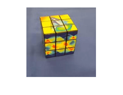
Load the example image. Save its size for future use.
imgFile = fullfile(pwd,'MerchData','MathWorks Cube','MathWorks cube_0.jpg');
inputImg = imresize(imread(imgFile),inputSize(1:2));
imshow(inputImg)
Show Activations of First Maxpool Layer
Investigate features by observing which areas in the convolution layers activate on an image. Compare that image to the corresponding areas in the original images. Each layer of a convolutional neural network consists of many 2-D arrays called channels. Pass the image through the network and examine the output activations of the pool1 layer.
act1 = simObj.activations(single(inputImg),'pool1');The activations are returned as a 3-D array, with the third dimension indexing the channel on the pool1 layer. To show these activations by using the imtile function, reshape the array to 4-D. The third dimension in the input to imtile represents the image color. Set the third dimension to have size 1 because the activations do not have color. The fourth dimension indexes the channel.
sz = size(act1);
act1 = reshape(act1,[sz(1) sz(2) 1 sz(3)]);
Display the activations. Each activation can take any value, so normalize the output by using the mat2gray. All activations are scaled so that the minimum activation is 0 and the maximum activation is 1. Display the 64 images on an 8-by-8 grid, one for each channel in the layer.
I = imtile(mat2gray(act1),'GridSize',[8 8]);
imshow(I)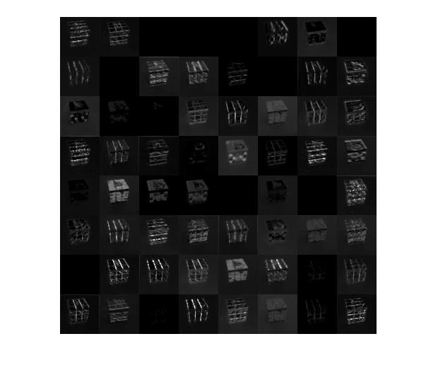
Find Strongest Activation Channel
Find the strongest channels by programmatically investigating channels with large activations. Find the channel that has the largest activation by using the max function, resize the channel output, and display the activations.
[maxValue,maxValueIndex] = max(max(max(act1)));
act1chMax = act1(:,:,:,maxValueIndex);
act1chMax = mat2gray(act1chMax);
act1chMax = imresize(act1chMax,inputSize(1:2));

I = imtile({inputImg,act1chMax});
imshow(I)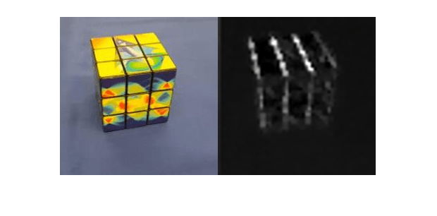
Compare the strongest activation channel image to the original image. This channel activates on edges. It activates positively on light left/dark right edges and negatively on dark left/light right edges.
Verify Prediction Results
Verify and display the prediction results of the dlhdl.Simulator object by using the predict function.
prediction = simObj.predict(single(inputImg));
[val, idx] = max(prediction);
netTransfer.Layers(end).ClassNames{idx}
ans = 'MathWorks Cube'
See Also
dlhdl.Simulator | activations | predict | dlhdl.ProcessorConfig
You can also select a web site from the following list:
Americas
- América Latina (Español)
- Canada (English)
- United States (English)
Europe
- Belgium (English)
- Denmark (English)
- Deutschland (Deutsch)
- España (Español)
- Finland (English)
- France (Français)
- Ireland (English)
- Italia (Italiano)
- Luxembourg (English)
- Netherlands (English)
- Norway (English)
- Österreich (Deutsch)
- Portugal (English)
- Sweden (English)
- Switzerland
- United Kingdom (English)