Analyze Shallow Neural Network Performance After Training
This topic presents part of a typical shallow neural network workflow. For more information and other steps, see Multilayer Shallow Neural Networks and Backpropagation Training. To learn about how to monitor deep learning training progress, see Monitor Deep Learning Training Progress.
When the training in Train and Apply Multilayer Shallow Neural Networks is complete,
you can check the network performance and determine if any changes need to be made to the
training process, the network architecture, or the data sets. First check the training record, tr, which was the second argument returned
from the training function.
tr
tr = struct with fields:
        trainFcn: 'trainlm'
      trainParam: [1×1 struct]
      performFcn: 'mse'
    performParam: [1×1 struct]
        derivFcn: 'defaultderiv'
       divideFcn: 'dividerand'
      divideMode: 'sample'
     divideParam: [1×1 struct]
        trainInd: [2 3 5 6 9 10 11 13 14 15 18 19 20 22 23 24 25 29 30 31 33 35 36 38 39 40 41 44 45 46 47 48 49 50 51 52 54 55 56 57 58 59 62 64 65 66 68 70 73 76 77 79 80 81 84 85 86 88 90 91 92 93 94 95 96 97 98 99 100 101 102 103 … ] (1×176 double)
          valInd: [1 8 17 21 27 28 34 43 63 71 72 74 75 83 106 124 125 134 140 155 157 158 162 165 166 175 177 181 187 191 196 201 205 212 233 243 245 250]
         testInd: [4 7 12 16 26 32 37 42 53 60 61 67 69 78 82 87 89 104 105 110 111 112 133 135 149 151 153 163 170 189 203 216 217 222 226 235 246 247]
            stop: 'Training finished: Met validation criterion'
      num_epochs: 9
       trainMask: {[NaN 1 1 NaN 1 1 NaN NaN 1 1 1 NaN 1 1 1 NaN NaN 1 1 1 NaN 1 1 1 1 NaN NaN NaN 1 1 1 NaN 1 NaN 1 1 NaN 1 1 1 1 NaN NaN 1 1 1 1 1 1 1 1 1 NaN 1 1 1 1 1 1 NaN NaN 1 NaN 1 1 1 NaN 1 NaN 1 NaN NaN 1 NaN NaN 1 1 NaN 1 1 1 … ] (1×252 double)}
         valMask: {[1 NaN NaN NaN NaN NaN NaN 1 NaN NaN NaN NaN NaN NaN NaN NaN 1 NaN NaN NaN 1 NaN NaN NaN NaN NaN 1 1 NaN NaN NaN NaN NaN 1 NaN NaN NaN NaN NaN NaN NaN NaN 1 NaN NaN NaN NaN NaN NaN NaN NaN NaN NaN NaN NaN NaN NaN NaN … ] (1×252 double)}
        testMask: {[NaN NaN NaN 1 NaN NaN 1 NaN NaN NaN NaN 1 NaN NaN NaN 1 NaN NaN NaN NaN NaN NaN NaN NaN NaN 1 NaN NaN NaN NaN NaN 1 NaN NaN NaN NaN 1 NaN NaN NaN NaN 1 NaN NaN NaN NaN NaN NaN NaN NaN NaN NaN 1 NaN NaN NaN NaN NaN … ] (1×252 double)}
      best_epoch: 3
            goal: 0
          states: {'epoch'  'time'  'perf'  'vperf'  'tperf'  'mu'  'gradient'  'val_fail'}
           epoch: [0 1 2 3 4 5 6 7 8 9]
            time: [3.9220 4.2656 4.2863 4.3209 4.4013 4.4196 4.4386 4.4460 4.4642 4.4790]
            perf: [672.2031 94.8128 43.7489 12.3078 9.7063 8.9212 8.0412 7.3500 6.7890 6.3064]
           vperf: [675.3788 76.9621 74.0752 16.6857 19.9424 23.4096 26.6791 29.1562 31.1592 32.9227]
           tperf: [599.2224 97.7009 79.1240 24.1796 31.6290 38.4484 42.7637 44.4194 44.8848 44.3171]
              mu: [1.0000e-03 0.0100 0.0100 0.1000 0.1000 0.1000 0.1000 0.1000 0.1000 0.1000]
        gradient: [2.4114e+03 867.8889 301.7333 142.1049 12.4011 85.0504 49.4147 17.4011 15.7749 14.6346]
        val_fail: [0 0 0 0 1 2 3 4 5 6]
       best_perf: 12.3078
      best_vperf: 16.6857
      best_tperf: 24.1796
This structure contains all of the information concerning the training of the network.
For example, tr.trainInd, tr.valInd and
tr.testInd contain the indices of the data points that were used in
the training, validation and test sets, respectively. If you want to retrain the network
using the same division of data, you can set net.divideFcn to
'divideInd', net.divideParam.trainInd to
tr.trainInd, net.divideParam.valInd to
tr.valInd, net.divideParam.testInd to
tr.testInd.
The tr structure also keeps track of several variables during the
course of training, such as the value of the performance function, the magnitude of the
gradient, etc. You can use the training record to plot the performance progress by using
the plotperf command:
plotperf(tr)
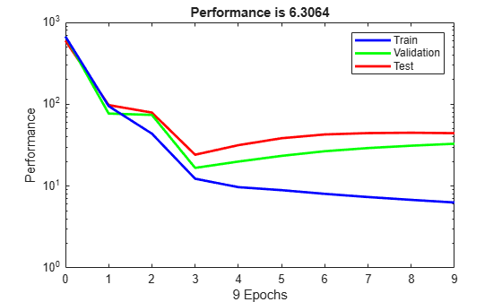
The property tr.best_epoch indicates the iteration at which the
validation performance reached a minimum. The training continued for 6 more iterations
before the training stopped.
This figure does not indicate any major problems with the training. The validation and test curves are very similar. If the test curve had increased significantly before the validation curve increased, then it is possible that some overfitting might have occurred.
The next step in validating the network is to create a regression plot, which shows the relationship between the outputs of the network and the targets. If the training were perfect, the network outputs and the targets would be exactly equal, but the relationship is rarely perfect in practice. For the body fat example, we can create a regression plot with the following commands. The first command calculates the trained network response to all of the inputs in the data set. The following six commands extract the outputs and targets that belong to the training, validation and test subsets. The final command creates three regression plots for training, testing and validation.
bodyfatOutputs = net(bodyfatInputs);
trOut = bodyfatOutputs(tr.trainInd);
vOut = bodyfatOutputs(tr.valInd);
tsOut = bodyfatOutputs(tr.testInd);
trTarg = bodyfatTargets(tr.trainInd);
vTarg = bodyfatTargets(tr.valInd);
tsTarg = bodyfatTargets(tr.testInd);
plotregression(trTarg, trOut, 'Train', vTarg, vOut, 'Validation', tsTarg, tsOut, 'Testing')
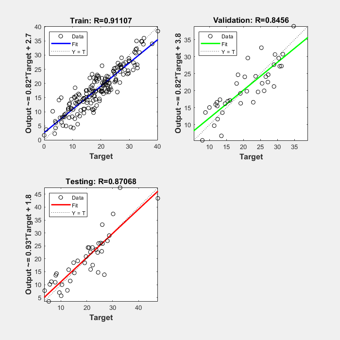
The three plots represent the training, validation, and testing data. The dashed line in each plot represents the perfect result – outputs = targets. The solid line represents the best fit linear regression line between outputs and targets. The R value is an indication of the relationship between the outputs and targets. If R = 1, this indicates that there is an exact linear relationship between outputs and targets. If R is close to zero, then there is no linear relationship between outputs and targets.
For this example, the training data indicates a good fit. The validation and test results also show large R values. The scatter plot is helpful in showing that certain data points have poor fits. For example, there is a data point in the test set whose network output is close to 35, while the corresponding target value is about 12. The next step would be to investigate this data point to determine if it represents extrapolation (i.e., is it outside of the training data set). If so, then it should be included in the training set, and additional data should be collected to be used in the test set.
Improving Results
If the network is not sufficiently accurate, you can try initializing the network and the training again. Each time your initialize a feedforward network, the network parameters are different and might produce different solutions.
net = init(net);
net = train(net, bodyfatInputs, bodyfatTargets);
As a second approach, you can increase the number of hidden neurons above 20. Larger numbers of neurons in the hidden layer give the network more flexibility because the network has more parameters it can optimize. (Increase the layer size gradually. If you make the hidden layer too large, you might cause the problem to be under-characterized and the network must optimize more parameters than there are data vectors to constrain these parameters.)
A third option is to try a different training function. Bayesian regularization
training with trainbr, for example, can sometimes
produce better generalization capability than using early stopping.
Finally, try using additional training data. Providing additional data for the network is more likely to produce a network that generalizes well to new data.