fitfepanel

R2026b

Fit one-way, linear, fixed-effects panel data regression model

Since R2026b

Syntax

EstMdl = fitfepanel(X,Y)

EstMdl = fitfepanel(X,Y,groups)

EstMdl = fitfepanel(Tbl,PredictorVariables=predictorVariables,GroupVariable=groupVariable)

EstMdl = fitfepanel(___,Name=Value)

Description

EstMdl = fitfepanel(X,Y) returns the one-way, linear, fixed-effects panel data regression model EstMdl from fitting the model to the input panel data in wide format. X is a T-by-n-by-p array of predictor data, Y is a T-by-n matrix of response data, where T is the greatest number of sampling time points among subjects, n is the number of sampled subjects, and p is the number of predictor variables. A data set in wide format must be organized as follows:

• Rows correspond to time points in the sample. That is, row t contains all p measurements for all n subjects at time t.

• Columns correspond to sampled subjects. That is, column c contains all p measurements over all T time points of subject c.

• For X, pages correspond to predictor variables. That is, page k contains measurements of predictor k for all n subjects and T time points in the sample. None of the predictors can represent an intercept. Among subjects, sampled time points correspond to each other (fitfepanel assumes all subjects are measured simultaneously).

EstMdl is a panel data regression model PanelModel.

EstMdl = fitfepanel(X,Y,groups) fits a fixed-effects model to the panel data in long format. X is an m-by-p matrix of predictor data. Y is an m-by-1 vector of response data, where m is the number of observations (for example, m = Tn for a balanced panel data set). Each row is an observation (all measurements) associated with a particular subject at a particular time, and each column is a variable. The groups input specifies the subject to which the observation belongs. For a subject, larger row indices indicate measurements taken later in the sample.

EstMdl = fitfepanel(Tbl,PredictorVariables=predictorVariables,GroupVariable=groupVariable) fits a fixed-effects model to the predictor, response, and subject-assignment data in the table or timetable Tbl. Panel data in a table is in long format. The Tbl input argument has m rows, and each row is an observation. The predictorVariables input specifies which table variables are predictor variables. groupVariable specifies the subject to which the measurements in the rows of data belong. The last table variable is the response variable, but you can specify a different variable as the response by using the ResponseVariable name-value argument.

EstMdl = fitfepanel(___,Name=Value) uses additional options specified by name-value arguments, and uses any input-argument combination in the previous syntaxes. For example, fitfepanel(Tbl,PredictorVariables=predictors,GroupVariable="Country",ResponseVariable="LogGDP",FitEffects=false,Method="difference") specifies that the table variable LogGDP contains the response data, the table variable Country contains the subject identifiers, and the arbitrary string vector predictors contains the predictor variable names in the table. This syntax does not fit the unobserved effects, and estimates the parameters using the first-difference transformation method.

Examples

Fit Fixed-Effects Model to Data in Wide Format

Fit a fixed-effects model to data using the default options. The data is in wide format.

Load the simulated, balanced panel data set Data_SimulatedBalancedPanel.mat, which is available when you open the live script for this example. The data set contains 12 microeconomic measurements of 1000 randomly selected people taken yearly from 2006 through 2020. The response variable in the model is a series of log wages, while all other variables in the data are predictors.

load Data_SimulatedBalancedPanel

For details on the data set, enter Description at the command line.

The variable Data is a 3-D numeric array containing the predictor and response variables. Each row is a time point in the sampling period, each column is a subject in the sample, and each page is a variable. The final variable in Data is the response variable (log wage series), while all other variables are predictors.

Create separate variables for the predictor and response data.

X = Data(:,:,1:(end-1));
Y = Data(:,:,end);

X is a 15-by-1000-by-11 numeric array of predictor data and Y is a 15-by-1000 numeric matrix. For example, X(10,501,3) is the education level of subject 501 in 2015.

Create a binary numeric variable for whether the subject is female (coded as 1) by using predictor 2, and a binary numeric variable for whether the subject is married (coded as 1) by using predictor 9.

X(:,:,2) = double(X(:,:,2) == 1);
X(:,:,9) = double(X(:,:,9) == 1);

Assume that the subject effect (heterogeneity) is associated with at least one of the predictor variables. Fit a fixed-effects model to the data sing the default options.

EstMdl = fitfepanel(X,Y);

Panel data information: 
Number of cross-sectional units (N):  1000
Number of periods (T):  15
Number of observations:  15000
Method of estimation:  fixed effects (within estimator)

          | Estimator    SE      tStat   pValue 
------------------------------------------------
 x1       |   0.0483   0.0003  143.2395   0     
 x2       |    0        0                       
 x3       |    0        0                       
 x4       |    0        0                       
 x5       |  -0.0618   0.0048  -12.9130  0.0000 
 x6       |   0.0097   0.0054    1.8055  0.0710 
 x7       |  -0.0261   0.0127   -2.0562  0.0398 
 x8       |  -0.0137   0.0075   -1.8337  0.0667 
 x9       |  -0.0695   0.0120   -5.7986  0.0000 
 x10      |   0.0740   0.0051   14.4116  0.0000 
 x11      |   0.0016   0.0003    5.7551  0.0000 
 variance |   0.0302                            

fitfepanel displays an estimation summary. For predictor j, row xj contains the coefficient estimate, standard error, and $t$ statistic for a two-tailed $t$ test that the coefficient is 0 with its $p$-value. All predictor variables, except for x6 and x8, are significant to the 5% significance level.

Coefficients associated with predictors x2, x3, and x4 are exactly 0 because they are time-invariant, demographics-based predictors. In fixed-effects models, the heterogeneity absorbs the effects of the predictors.

Display the fitted model.

EstMdl

EstMdl = 
  PanelModel with properties:

             Coefficients: [11×1 double]
    CoefficientCovariance: [11×11 double]
      DisturbanceVariance: 0.0302
           EffectVariance: Inf
                  Effects: [5.4228 5.5360 5.6740 6.3112 6.1355 6.2778 5.0113 6.4766 6.0565 5.2756 6.2547 5.4123 6.1649 5.6834 5.1302 5.6340 5.7004 5.9854 5.3196 4.6600 4.8870 5.7634 5.7455 5.3122 5.9827 5.4779 6.2823 4.8012 5.3795 … ] (1×1000 double)
            LogLikelihood: 5.4849e+03
                  Summary: [12×4 table]
                     Type: "FixedEffects"

EstMdl is a PanelModel object. You can access its properties using dot notation.

Plot the empirical distribution of the heterogeneity.

effects = EstMdl.Effects;
histogram(effects,Normalization="probability")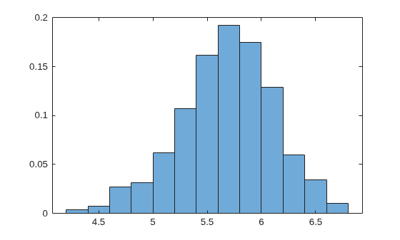

Fit Fixed-Effects Model to Data in Long Format

Fit a fixed-effects model to data using default options. The data is in long format.

Load the simulated, balanced panel data set Data_SimulatedBalancedPanel.mat, which is available when you open the live script for this example. The data set contains 12 microeconomic measurements of 1000 randomly selected people taken yearly from 2006 through 2020. The response variable in the model is a series of log wages, while all other variables in the data are predictors.

Load and Extract Data

load Data_SimulatedBalancedPanel

For details on the data set, enter Description at the command line.

The variable Data is a 3-D numeric array containing the predictor and response variables. Each row is a time point in the sampling period, each column is a subject in the sample, and each page is a variable. The final variable in Data is the response variable (log wage series), while all other variables are predictors. This data is in wide format.

Create separate variables for the predictor and response data. Determine the time span of the sample $T$, the number of subjects $n$, and the number of predictor variables $p$.

X = Data(:,:,1:(end-1));
Y = Data(:,:,end);
[T,n,p] = size(X)

T = 
15

n = 
1000

p = 
11

X is a 15-by-1000-by-11 numeric array of predictor data and Y is a 15-by-1000 numeric matrix. For example, X(10,501,3) is the education experience of subject 501 in 2015.

Convert Data to Long Format

Data in long format must have the following characteristics:

• The response data is a $Tn$-by-1 vector. In this example, the long format response data is a 15000-by-1 vector.

• The predictor data is a $Tn$-by-$p$ matrix. In this example, the long format predictor data is a 15000-by-11 matrix.

• The software must be able to identify which subject the observation belongs to using a $Tn$-by-1 vector of subject IDs.

• For each subject, the software assumes that observations in higher rows were sampled later than observations in lower rows.

Convert the response data to long format by stacking the columns of Y using linear indexing with a single colon.

YLong = Y(:);
size(YLong)

ans = 1×2

       15000           1

For selected subjects, verify that the responses are arranged by blocks of subjects, increasing by sampling time within each block. To choose a subject to check, use the control.

j = 3; % Subject index
YSubj = Y(1:T,j);
YLongSubj = YLong((T*(j-1)+1):(T*j));
sum(YSubj - YLongSubj)

ans = 
0

Convert the predictor data to long format by stacking the columns of X and setting its pages to columns using reshape.

XLong = reshape(X,T*n,11);
size(XLong)

ans = 1×2

       15000          11

XLong is arranged such that all subject-specified measurements are blocked together and stacked, and within-subject blocks of observations are arranged in increasing order by sampling time.

For selected subjects, verify that the predictor data is arranged by blocks of subjects, increasing by sampling time within each block. To choose a subject to check, use the control. After choosing the subject, collapse the 3-D data into a matrix by using the squeeze function.

j = 6; 
XSubj = squeeze(X(1:T,j,:));
XLongSubj = XLong((T*(j-1)+1):(T*j),:);
sum(sum(XSubj - XLongSubj))

ans = 
0

Observations are arranged by blocks of subjects. Create a numeric vector that identifies each subject by repeating each integer in the interval $\left[1,n\right]$ $T$ times, and then stacking the results.

Groups = repmat(1:n,T,1);
Groups = Groups(:);

Preprocess Data

Create a binary numeric variable for whether the subject is female (coded as 1) by using predictor 2, and a binary numeric variable for whether the subject is married (coded as 1) by using predictor 9.

XLong(:,2) = double(XLong(:,2) == 1);
XLong(:,9) = double(XLong(:,9) == 1);

Fit Model to Data

Assume that the heterogeneity is associated with at least one of the predictor variables. Fit a fixed-effects model to the data in long format using the default options. Specify the grouping variable.

EstMdl = fitfepanel(XLong,YLong,Groups);

Panel data information: 
Number of cross-sectional units (N):  1000
Number of periods (T):  15
Number of observations:  15000
Method of estimation:  fixed effects (within estimator)

          | Estimator    SE      tStat   pValue 
------------------------------------------------
 x1       |   0.0483   0.0003  143.2395   0     
 x2       |    0        0                       
 x3       |    0        0                       
 x4       |    0        0                       
 x5       |  -0.0618   0.0048  -12.9130  0.0000 
 x6       |   0.0097   0.0054    1.8055  0.0710 
 x7       |  -0.0261   0.0127   -2.0562  0.0398 
 x8       |  -0.0137   0.0075   -1.8337  0.0667 
 x9       |  -0.0695   0.0120   -5.7986  0.0000 
 x10      |   0.0740   0.0051   14.4116  0.0000 
 x11      |   0.0016   0.0003    5.7551  0.0000 
 variance |   0.0302                            

Fit Fixed-Effects to Data in Timetable

Fit a fixed-effects model to data using the default options. The data is in a timetable.

Load the simulated, balanced panel data set Data_SimulatedBalancedPanel.mat, which is available when you open the live script for this example. The data set contains 12 microeconomic measurements of 1000 randomly selected people taken yearly from 2006 through 2020. The response variable in the model is a series of log wages, while all other variables in the data are predictors.

load Data_SimulatedBalancedPanel

For details on the data set, enter Description at the command line.

The variable DataTimeTable is a timetable containing the data. LogWage is the response variable, Group is the subject ID (grouping) variable, and all other variables are predictors. Each row is an observation for a subject at a time point in the sampling period (in other words, this data format is long).

Display the head and size of the timetable of data.

head(DataTimeTable)

    Time    WorkExperience    Gender    Education    Ethnicity    IsBlueCollar    IsManufacturing    IsSouth    IsCity    MaritalStatus    IsUnion    WeeksWorked    Group    LogWage
    ____    ______________    ______    _________    _________    ____________    _______________    _______    ______    _____________    _______    ___________    _____    _______

    2006          29          female       12            0             1                 0              0         0       nevermarried        0           48           1      6.7956 
    2007          30          female       12            0             1                 0              0         0       nevermarried        0           49           1      6.6592 
    2008          31          female       12            0             1                 0              0         0       nevermarried        0           51           1      6.9801 
    2009          32          female       12            0             0                 0              0         0       nevermarried        0           45           1      7.2397 
    2010          33          female       12            0             0                 0              0         0       nevermarried        0           25           1       7.123 
    2011          34          female       12            0             0                 0              0         0       nevermarried        0           42           1      6.9183 
    2012          35          female       12            0             0                 0              0         0       nevermarried        0           48           1      7.1639 
    2013          36          female       12            0             0                 0              0         0       nevermarried        0           49           1      7.0534 

size(DataTimeTable)

ans = 1×2

       15000          13

Create a new timetable TT containing a binary numeric variable for whether the subject is female by using Gender, and a binary numeric variable for whether the subject is married by using MaritalStatus. Then, remove the corresponding variables from TT.

TT = DataTimeTable;
TT.IsFemale = double(TT.Gender == "female");
TT = movevars(TT,"IsFemale","Before","Gender");
TT.Gender = [];
TT.IsMarried = double(TT.MaritalStatus == "married");
TT = movevars(TT,"IsMarried","Before","MaritalStatus");
TT.MaritalStatus = [];

Fit a fixed-effects model of the log wage series (LogWage) to all other variables, except the subject ID (Group), in the timetable. Specify the predictor and grouping variable names. fitfepanel assumes that the final variable is the response variable.

prednames = TT.Properties.VariableNames(1:end-2);
EstMdl = fitfepanel(TT,PredictorVariables=prednames,GroupVariable="Group");

Panel data information: 
Number of cross-sectional units (N):  1000
Number of periods (T):  15
Number of observations:  15000
Method of estimation:  fixed effects (within estimator)

                 | Estimator    SE      tStat   pValue 
-------------------------------------------------------
 WorkExperience  |   0.0483   0.0003  143.2395   0     
 IsFemale        |    0        0                       
 Education       |    0        0                       
 Ethnicity       |    0        0                       
 IsBlueCollar    |  -0.0618   0.0048  -12.9130  0.0000 
 IsManufacturing |   0.0097   0.0054    1.8055  0.0710 
 IsSouth         |  -0.0261   0.0127   -2.0562  0.0398 
 IsCity          |  -0.0137   0.0075   -1.8337  0.0667 
 IsMarried       |  -0.0695   0.0120   -5.7986  0.0000 
 IsUnion         |   0.0740   0.0051   14.4116  0.0000 
 WeeksWorked     |   0.0016   0.0003    5.7551  0.0000 
 variance        |   0.0302                            

Fit Model Using First-Difference Transformation Method

Estimate a fixed-effects model of log wages as a function of a set of predictors by applying the first-difference transformation method. By default, fitfepanel uses the "within-transformation" method to estimate the model.

Load the simulated, balanced panel data set Data_SimulatedBalancedPanel.mat, which is available when you open the live script for this example. The data set contains 12 microeconomic measurements of 1000 randomly selected people taken yearly from 2006 through 2020. The response variable in the model is a series of log wages, while all other variables in the data are predictors.

load Data_SimulatedBalancedPanel

For details on the data set, enter Description at the command line.

Create a new timetable TT containing a binary numeric variable for whether the subject is female by using Gender, and a binary numeric variable for whether the subject is married by using MaritalStatus. Then, remove the corresponding variables from TT.

TT = DataTimeTable;
TT.IsFemale = double(TT.Gender == "female");
TT = movevars(TT,"IsFemale","Before","Gender");
TT.Gender = [];
TT.IsMarried = double(TT.MaritalStatus == "married");
TT = movevars(TT,"IsMarried","Before","MaritalStatus");
TT.MaritalStatus = [];

Fit a fixed-effects model of the log wage series (LogWage) to all other variables, except the subject ID, in the processed timetable TT. Specify the first-difference transformation estimation method.

varnames = TT.Properties.VariableNames;
prednames = varnames(~ismember(varnames,["Group" "LogWage"]));
EstMdl = fitfepanel(TT,PredictorVariables=prednames,GroupVariable="Group",Method="difference"); 

Panel data information: 
Number of cross-sectional units (N):  1000
Number of periods (T):  15
Number of observations:  15000
Method of estimation:  fixed effects (difference estimator)

                 | Estimator    SE     tStat   pValue 
------------------------------------------------------
 WorkExperience  |   0.0485   0.0021  23.2563  0.0000 
 IsFemale        |    0        0                      
 Education       |    0        0                      
 Ethnicity       |    0        0                      
 IsBlueCollar    |  -0.0597   0.0093  -6.4507  0.0000 
 IsManufacturing |  -0.0011   0.0108  -0.0982  0.9218 
 IsSouth         |  -0.0291   0.0296  -0.9806  0.3268 
 IsCity          |  -0.0127   0.0160  -0.7942  0.4271 
 IsMarried       |  -0.0898   0.0278  -3.2339  0.0012 
 IsUnion         |   0.0610   0.0103   5.9193  0.0000 
 WeeksWorked     |   0.0017   0.0003   6.1182  0.0000 
 variance        |   0.0605                           

The results using the within-transformation method are different from the default method. At the 10% significance level, all coefficients resulting from using the default method are significant, but the within-method results in insigificant coefficients associates with IsManufacturing, IsSouth, and IsCity.

Obtain Robust Estimates from Fixed-Effects Regression

Fit a fixed-effects model to data and obtain robust estimates.

Load the simulated, balanced panel data set Data_SimulatedBalancedPanel.mat, which is available when you open the live script for this example. The data set contains 12 microeconomic measurements of 1000 randomly selected people taken yearly from 2006 through 2020. The response variable in the model is a series of log wages, while all other variables in the data are predictors.

load Data_SimulatedBalancedPanel

For details on the data set, enter Description at the command line.

Create separate variables for the predictor and response data. Determine the time span of the sample $T$, the number of subjects $n$, and the number of predictor variables $p$.

X = Data(:,:,1:(end-1));
[T,n,p] = size(X);
Y = Data(:,:,end);

Create a binary numeric variable for whether the subject is female (coded as 1) by using predictor 2, and a binary numeric variable for whether the subject is married (coded as 1) by using predictor 9.

X(:,:,2) = double(X(:,:,2) == 1);
X(:,:,9) = double(X(:,:,9) == 1);

Simulate heteroscedasticity in the system by using unmeasured, subject-specific predictor variables $z_j$ such that, for each subject $j=1,...,n$, $z_j\sim Pois\left({\lambda }_j\right)$ and ${\lambda }_j\sim Uniform\left(1,...,50\right)$. For each subject, simulate $T$ values.

rng(1,"twister")
Z = zeros(T,n);
for j = 1:n
    lambda = randi(50);
    Z(:,j) = poissrnd(lambda,T,1);
end

Add the simulated predictor data to the response data with coefficient ${\beta }_z=2$.

YSim = Y + 2*Z;

Assume that the heterogeneity is associated with at least one of the predictor variables. Fit a fixed effects model to the predictor data without $z$, but supply the simulated response data. Use the default options.

EstMdl = fitfepanel(X,YSim);

Panel data information: 
Number of cross-sectional units (N):  1000
Number of periods (T):  15
Number of observations:  15000
Method of estimation:  fixed effects (within estimator)

          | Estimator    SE     tStat   pValue 
-----------------------------------------------
 x1       |    0.0168  0.0196   0.8563  0.3918 
 x2       |     0       0                      
 x3       |     0       0                      
 x4       |     0       0                      
 x5       |    0.3551  0.2780   1.2774  0.2015 
 x6       |   -0.2190  0.3109  -0.7044  0.4812 
 x7       |    0.9388  0.7386   1.2710  0.2037 
 x8       |    0.1095  0.4337   0.2526  0.8006 
 x9       |    0.2667  0.6960   0.3832  0.7016 
 x10      |   -0.0456  0.2984  -0.1529  0.8784 
 x11      |    0.0068  0.0162   0.4227  0.6725 
 variance |  101.9401                          

Compute the model residuals $${\underset{}{\overset{ˆ}{\epsilon }}}_{ti}=Y_{ti}-X_{ti}\underset{}{\overset{ˆ}{\beta }}-{\underset{}{\overset{ˆ}{\alpha }}}_i$$ and plot them against the fitted responses. Color the residuals according to subject ID.

betahat = reshape(EstMdl.Coefficients,1,1,p);
alphahat = EstMdl.Effects;
Yhat = sum(X.*betahat,3) + alphahat;
Residuals = YSim - Yhat;
figure
plot(Yhat,Residuals,'.')
hold on
yline(0,"--")
hold off
title("Residuals by Subject")
ylabel("Residual")
xlabel("Fitted Value")

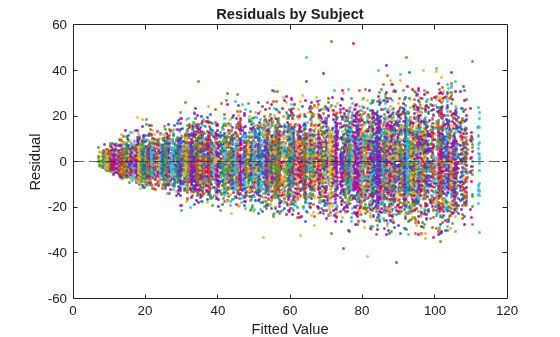
The residuals scatter more widely as the fitted values increase. This behavior is indicative of heteroscedasticity. Also, the residuals appear clustered by groups.

Refit the model and compute robust covariance estimates.

EstMdlRobust = fitfepanel(X,YSim,RobustCovariance=true);

Panel data information: 
Number of cross-sectional units (N):  1000
Number of periods (T):  15
Number of observations:  15000
Method of estimation:  fixed effects (within estimator)

          | Estimator    SE     tStat   pValue 
-----------------------------------------------
 x1       |    0.0168  0.0197   0.8525  0.3939 
 x2       |     0       0                      
 x3       |     0       0                      
 x4       |     0       0                      
 x5       |    0.3551  0.2781   1.2769  0.2017 
 x6       |   -0.2190  0.3239  -0.6760  0.4990 
 x7       |    0.9388  0.7077   1.3266  0.1846 
 x8       |    0.1095  0.4425   0.2475  0.8045 
 x9       |    0.2667  0.6889   0.3871  0.6987 
 x10      |   -0.0456  0.3001  -0.1520  0.8791 
 x11      |    0.0068  0.0159   0.4300  0.6672 
 variance |  101.9401                          

The coefficient estimates between the robust and nonrobust runs are the same; the difference between the runs is in the inferences.

Plot a heatmap of the difference between the estimated coefficient covariance matrices.

seriesSim = series(1:p);
heatmap(seriesSim,seriesSim,(EstMdlRobust.CoefficientCovariance-EstMdl.CoefficientCovariance)./EstMdl.CoefficientCovariance)

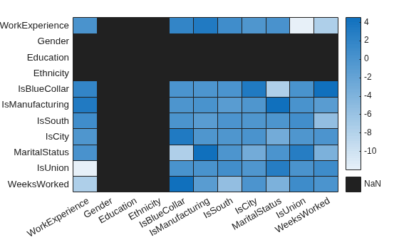
The estimated covariance of the coefficients of WorkExperience and IsUnion shows the greatest relative difference between the robust and nonrobust analyses.

Input Arguments

X — Predictor data X

numeric matrix | numeric 3-D array

Predictor data X, specified as an m-by-p numeric matrix or a T-by-n-by-p numeric 3-D array, where m is the total number of observations, p is the number of predictor variables, n is the number of sampled subjects (groups), and T is the largest number of sampling time points among subjects.

When X is a matrix, the data sets are in long format and the following conditions apply:

• You must provide the input groups, which identifies the subjects.

• Each row is an observation taken at a particular time from a particular subject. That is, row j contains the measurements for all predictors at time t for the subject g, where groups(j) is g.

• Suppose Xg = X(groups == g,:) identifies the observations of subject g. Thus, row t1 < row t1 implies Xg(t1,:) was observed earlier than Xg(t2,:).

• For each sampling time t, fitfepanel assumes that all subjects were measured simultaneously.

• Column k contains the measurements of predictor variable k.

• You must provide the response data Y as an m-by-1 vector.

When X is a 3-D array, the data sets are in wide format and the following conditions apply:

• Row t contains all the measurements taken at time t. Row t₁ < row t₂ implies the sampling time t₁ < sampling time t₂.

• Column c contains all the measurements of subject c.

• Page k contains the measurements of predictor variable k.

• You must provide the response data Y as a T-by-n matrix.

Do not include a predictor variable entirely composed of ones in X to represent the model intercept.

NaN values in X indicate missing measurements. For unbalanced data in wide format, you must insert rows of NaN values for unmeasured time points among all pages.

For more details, see Panel Data.

Data Types: double

Y — Response data Y

numeric vector | numeric matrix

Response data Y, specified as an m-by-1 numeric vector or a T-by-n numeric matrix.

When Y is a vector, the data sets are in long format and the following conditions apply:

• You must provide the input groups, which identifies the subjects.

• Row j contains the response at time t for the subject g, where input groups(j) is g.

• Suppose Yg = Y(groups == g) identifies the responses of subject g. Thus, fitfepanel assumes that, if Yg(j) was observed at time t, Yg(j + 1) was observed at time t + f, where f is the sampling frequency.

• For each sampling time t, fitfepanel assumes that all subjects were measured simultaneously.

• You must provide the predictor data X as an m-by-p matrix.

When Y is a matrix, the data sets are in wide format and the following conditions apply:

• Row t contains all the measurements taken at time t. Row t₁ < row t₂ implies the sampling time t₁ < sampling time t₂.

• Column c contains all the measurements of subject c.

• You must provide the predictor data X as a T-by-n-by-p 3-D array.

NaN values in Y indicate missing responses. For unbalanced data in wide format, you must insert rows of NaN values for unmeasured time points.

For more details, see Panel Data.

Data Types: double

groups — Subject (group) identifiers

vector

Subject (group) identifiers for unobserved effects, specified as an m-by-1 vector. The unique values in groups identify the sampled subjects.

When you specify data in long format, you must specify groups.

NaN values in groups indicate missing group identifiers for the corresponding observations. fitfepanel assigns such observations to an arbitrary group outside the set of known groups. This reassignment can result in unbalanced panel data.

For more details, see Panel Data.

Data Types: double | categorical | cell | char | string

Tbl — Panel data

table | timetable

Panel data in long format, to which fitfepanel fits the model, specified as a table or timetable with numvars = width(Tbl) variables and m = height(Tbl) rows.

When you specify Tbl, the following conditions apply:

• Each row is an observation taken at a particular time from a particular subject. That is, row j contains the measurements for all variables at time t for the subject g.

• Suppose Tblg = Tbl(Tbl.groupVariable == g,:) identifies the observations of subject g. Thus, fitfepanel assumes that, if Tblg(j,:) was observed at time t, Tblg(j + 1,:) was observed at time t + f, where f is the sampling frequency.

• For each sampling time t, fitfepanel assumes that all subjects were measured simultaneously.

• Specify the predictor variables in the model X by setting PredictorVariables=predictorVariables. Each selected predictor variable must be a numeric vector.

• Specify the subject (group) identifier variable by setting GroupVariable=groupVariable. The selected subject identifier variable can be a numeric, categorical, or string vector.

• By default, the last variable is the response variable Y, but you can specify a different variable by setting the ResponseVariable name-value argument. The selected response variable must be a numeric vector.

Do not include a predictor variable entirely composed of ones in Tbl to represent the model intercept.

NaN values in Tbl indicate missing measurements for the corresponding observations. fitfepanel removes entire observations from the data when it cannot assign them to a group. Such data removal can cause unbalanced panel data.

For more details, see Panel Data.

predictorVariables — Predictor variables X to select from Tbl

string vector | cell vector of character vectors | vector of integers | logical vector

Predictor variables X (which contain predictor data) to select from Tbl, specified as one of the following data types:

• String vector or cell vector of character vectors containing p variable names in Tbl.Properties.VariableNames

• A length p vector of unique indices (positive integers) of variables to select from Tbl.Properties.VariableNames

• A length numvars = width(Tbl) logical vector, where PredictorVariables(j) = true selects variable j from Tbl.Properties.VariableNames, and sum(PredictorVariables) is p

Example: ["M1SL" "TB3MS" "UNRATE"]

Example: [true false true false] or [1 3] selects the first and third table variables to supply the predictor data.

Data Types: double | logical | char | cell | string

groupVariable — Subject (group) variable to select from Tbl

string scalar | character vector | integer | logical vector

Subject (group) variable (which contains subject identifier data for the unobserved effects) to select from Tbl, specified as one of the following data types:

• String scalar or character vector containing the variable name to select from Tbl.Properties.VariableNames

• Variable index (positive integer) to select from Tbl.Properties.VariableNames

• A logical vector, where groupVariable(j) = true selects variable j from Tbl.Properties.VariableNames

Example: "Country"

Example: [false false true false] or 3 selects the third table variable as the subject variable.

Data Types: double | logical | char | cell | string

Name-Value Arguments

Specify optional pairs of arguments as Name1=Value1,...,NameN=ValueN, where Name is the argument name and Value is the corresponding value. Name-value arguments must appear after other arguments, but the order of the pairs does not matter.

Example: fitfepanel(Tbl,PredictorVariables=predictors,GroupVariable="Subjects",ResponseVariable="Response",FitEffects=false,Method="difference") specifies that the table variable "Response" contains the response data, the table variable "Subjects" contains the subject identifiers, and the arbitrary string vector predictors contains the predictor variable names in the table. This syntax does not fit the unobserved effects, and estimates the parameters using the first-difference transformation method.

Method — Parameter estimation method

"within" (default) | "difference"

Parameter estimation method, specified as "within" for the within transformation method and "difference" for the first-difference transformation method [1].

The "difference" method is more efficient than "within" when the disturbance series exhibits moderate to high serial correlation. Otherwise, the "within" method is more efficient.

For more details, see Estimation Method Descriptions.

Example: Method="difference"

Data Types: char | string

RobustCovariance — Robust covariance estimation flag

false (default) | true

Robust covariance estimation flag, specified as false or true.

Value	Description
false	fitfepanel does not compute cluster-robust covariance estimates.
true	fitfepanel computes cluster-robust covariance estimates.

Coefficient estimates between the nonrobust-covariance and robust-covariance estimation methods are equal. Coefficient covariance estimates and, therefore, inferences between the nonrobust and robust-covariance estimation methods are not necessarily equal.

Tip

Although you should set RobustCovariance=true when residuals show evidence of heteroscedasticity or serial correlation, [1] suggests using this setting whenever feasible.

Example: RobustCovariance=true

Data Types: logical

FitEffects — Unobserved effects ɑ estimation flag

true (default) | false

Unobserved effects ɑ estimation flag, specified as false or true.

Value	Description
false	fitfepanel does not estimate ɑ.
true	fitfepanel estimates ɑ and reports its estimates.

To fit the model using fewer computational resources and to obtain only coefficient and covariance estimates and inferences, set FitEffects=false.

For details, see Latent Effects Estimation.

Example: FitEffects=false

Data Types: logical

VarNames — Predictor variable names

string vector | cell vector of character vectors

Predictor variable names for display when you specify X, specified as a string vector or cell vector of character vectors. VarNames must contain p elements. VarNames(j) is the name of the variable j in the predictor data X.

When you specify a table or timetable of data Tbl, fitfepanel ignores VarNames and labels the predictor variables using the associated names in Tbl.Properties.VariableNames.

The default is ["x1" "x2" ... "xp"].

Example: VarNames=["UnemploymentRate"; "CPI"]

Data Types: string | cell | char

Display — Estimation display flag

true (default) | false

Estimation display flag, specified as true or false.

Value	Description
false	fitfepanel does not display estimation results to the command line.
true	fitfepanel displays estimation results to the command line.

Example: Display=false

Data Types: logical

ResponseVariable — Response variable y to select from Tbl

string scalar | character vector | integer | logical vector

Response variable y (which contains the response data) to select from Tbl, specified as one of the following data types:

• String scalar or character vector containing a variable name in Tbl.Properties.VariableNames

• Variable index (integer) to select from Tbl.Properties.VariableNames

• A length numvars logical vector, where ResponseVariable(j) = true selects variable j from Tbl.Properties.VariableNames, and sum(ResponseVariable) is 1

Example: ResponseVariable="Wages"

Example: ResponseVariable=[false false true false] or ResponseVariable=3 selects the third table variable as the response variable.

Data Types: double | logical | char | cell | string

Output Arguments

EstMdl — Estimated panel model

PanelModel object

Estimated panel model, returned as a PanelModel object. EstMdl contains properties that store the estimation results from fitting the fixed-effects model to the data. You can access the properties by using dot notation.

The fixed-effects model is the limiting case of the random effects panel regression model. Therefore, as the variance of the heterogeneity approaches infinity, the effect variance EstMdl.EffectVariance is Inf.

More About

Panel Data

A panel data set contains the measurements of n subjects measured at most T times over a sampling time frame. Panel data is a type of longitudinal data resulting from an observational study, rather than a controlled experiment. This distinction affects regression procedures used to analyze these types of data sets. (To analyze longitudinal data, see fitlme, fitlmematrix, and fitrm.)

You can format panel data sets in wide format or long format. In the following discussion, an observation is all measurements (predictors x_i, i = 1,…,p and response y data) of a subject (g_k, k = 1,...,n) at a particular time (t_j, j = 1,…,T).

In wide format, the predictor data set X (input X) is a T-by-n-by-p 3-D numeric array, where rows correspond to contemporaneous sampling times in increasing order by row, columns correspond to individual subjects, and pages correspond to predictor variables. The response data set Y (input Y) in wide format is a T-by-n matrix. The figure below illustrates the predictor and response data in wide format.

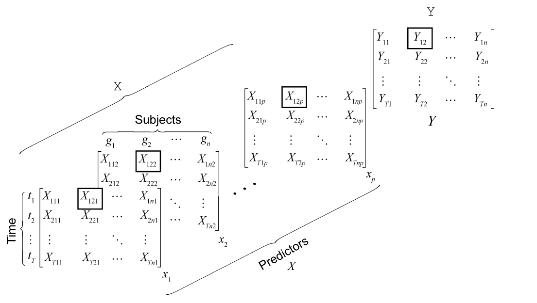
For a data set in this format, you can clearly infer the sampling time and subject by the corresponding row and column, respectively. An observation of subject g_k at time t_j is the set {X(j,k,:), Y(j,k)}. For example, the boxed values in the figure comprise the observation of subject g₂ at time t₁.

In long format, the predictor data set X is an m-by-p matrix, where $$m={\displaystyle \sum _{j=1}^n{T}_j},$$ the total sample size. Each row contains all predictor measurements of a particular subject at a particular time, and each column is a predictor variable. The response data set y is an m-by-1 vector, where each row is the response of the corresponding subject at the corresponding time. For data in this format, you cannot infer the subject and sampling time to which each observation belongs. A variable of subject identifiers (group variable), an m-by-1 vector, is required. For each subject, observations are recorded in increasing order by row. The figure below illustrates the predictor and response data in long format.

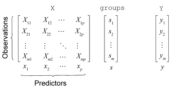
Row j of the subject identifier vector s_j is in the set {g₁,g₂,…,g_n}. This figure illustrates the variables for all observations of subject g₂ (s = g₂, coded as g2). In the figure, t_j = t(j). Because only those observations belonging to subject g ₂ are displayed, the row indices are not clear, but the sampling times are clear and, therefore, labeled.

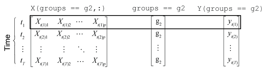
An observation of subject g_k at time t_j is the set {Xgk(j,:), Ygk(j)}, where Xgk = X(groups == gk,:) and Ygk = Y(groups == gk). For example, the boxed values in the figure comprise the observation of subject g₂ at time t₁.

A panel data set in a table or timetable is in long format. The Time variable of a timetable specifies the sampling times of the observations.

Regardless of format, when the data set contains the measurements for all subjects and sampling times, the data set is balanced. Otherwise, the data set is unbalanced.

One-way, Linear, Fixed-Effects Panel Data Regression Model

A one-way, linear, fixed-effects panel data regression model is a linear regression model for panel data that includes a term, called the fixed-effect, representing the influence of subjects on the response variable. The goals of a fixed-effects model are to study the impact of predictor variables on a response while controlling for latent, subject-specific effects, called heterogeneity, and to study the influence of the heterogeneity itself. Unlike in random-effects panel data regression models, the heterogeneity is correlated with at least one of the predictor variables.

A fixed-effects model resembles a typical linear random-effects model, with the following differences:

• Panel data is the result of an observational study, whereas data analyzed by a typical linear random-effects model is the result of an experimental study.

• Panel data analysis includes a study of the values of the heterogeneity. This goal is atypical for experimental studies, where an ANOVA is typically the goal.

Symbolically, the fixed-effects model is

$$y_{tj}=x_{tj}\prime \beta +{\alpha }_j+{\epsilon }_{tj},$$

where:

• y_tj is the scalar response (dependent variable) of subject (entity or group) j at time t, j = 1,…,n and t = 1,…,T.

• x_tj is a p-by-1 vector of the measurements of predictor variables (independent variables) of subject j at time t. x_tj does not contain a constant term for the intercept.

• β is a p-by-1 vector of fixed linear regression coefficients associated with the predictor variables. For each k = 1,…,p, coefficient k represents the influence predictor k averaged over all subjects and sampling times.

• ɑ_j is the scalar time-invariant heterogeneity of subject j, which is treated as a fixed effect. For each j = 1,…,n, ɑ_j represents the latent influence of subject j.

• ε_tj is the disturbance, or idiosyncratic error, of subject j at time t. The conditional distribution of ε_tj, given the predictors and heterogeneity, has a mean of 0 and variance σ²_ε.

• In addition to the usual linear model assumptions, fixed-effects models assume that the heterogeneity is endogenous, meaning that it is correlated with at least one predictor variable.

Because the heterogeneity is endogenous, ordinary least squares (OLS), with dummy-variable subject coding, produces inconsistent coefficient estimates. Without instrumental variables (which is a popular approach to estimating fixed-effects models), the within or first-difference transformation method estimates coefficients and the heterogeneity terms, and performs inference. For more details, see panel data.

Algorithms

Estimation Method Descriptions

fitfepanel supports the two parameter estimation methods described below (for more details, see [1]). The data must be complete for at least two sampling times.

• When Method is "within", fitfepanel uses the within transformation (fixed-effects transformation) method to transform the model. The method can be viewed as a dummy variable least squares (LSDV) model, where the predictor data matrix is augmented by a dummy variable matrix identifying the subject of the observation. In this case, the method estimates the coefficients and heterogeneity simultaneously. However, to avoid composing a large matrix in memory, LSDV can be accomplished in two stages. This algorithm summarizes the two-stage estimation procedure:

  1. Obtain a cross-section model by averaging over time.

     $${\overline{y}}_j={\overline{x}}_j\beta +{\alpha }_j+{\overline{\epsilon }}_j,$$

     where $${\overline{\epsilon }}_j={\displaystyle \sum _{t=1}^T{\epsilon }_{tj}}$$, $${\overline{x}}_j=\left[\begin{array}{cccc}{\overline{x}}_{j1}& {\overline{x}}_{j2}& \cdots & {\overline{x}}_{jp}\end{array}\right]={\displaystyle \sum _{t=1}^T\left[\begin{array}{cccc}{x}_{tj1}& x_{tj2}& \cdots & x_{tjp}\end{array}\right]}$$, and $${\overline{\epsilon }}_j={\displaystyle \sum _{t=1}^T{\epsilon }_{tj}}$$.

     Observe that the linear parameters are invariant to the transformation.

  2. Eliminate the heterogeneity by subtracting the cross-section model from the full model.

     $$\begin{array}{l}{y}_{tj}-{\overline{y}}_j=\left(x_{tj}-{\overline{x}}_j\right)\beta +{\epsilon }_{tj}-{\epsilon }_j\\ \Rightarrow {\tilde{y}}_{tj}={\tilde{x}}_{tj}\beta +{\tilde{\epsilon }}_{tj}.\end{array}$$

     Note the following:

     • The transformation has a form suitable for pooled ordinary least squares (OLS).

     • Time-invariant predictor variables are uninformative because their values are 0 for all t and j.

  3. To estimate β and σ²_ε, fit the transformed model to the data by applying pooled OLS. Coefficients of time-invariant predictors are 0. The variance estimator

     $${\widehat{\sigma }}_{\epsilon }^2=\frac{{\displaystyle {\sum }_j{\displaystyle {\sum }_t{\left({\tilde{y}}_{tj}-{\tilde{x}}_{tj}\widehat{\beta }\right)}^2}}}{M-n-p_1}$$

     is unbiased for σ²_ε. Note that the degrees of freedom is further reduced by n because this method, although two-stage, is equivalent to LSDV, where the n homogeneity terms are estimated with the coefficients. p₁ is the number of time-varying predictors, and the total sample size is $$M={\displaystyle {\sum }_{j=1}^n{T}_j}$$.

  4. The heterogeneity estimates are

     $${\widehat{\alpha }}_j=\frac{1}{T_j}{\displaystyle \sum _{t=1}^T\left(y_{tj}-x_{tj}\widehat{\beta }\right)},$$

     where $$\widehat{\beta }$$ is the pooled OLS estimate of β.

• When Method is "difference", fitfepanel uses the first-difference transformation method to transform the model. This method explicitly treats the parameters ɑ_j as nuisance parameters during the estimation of the coefficients, and then estimates each ɑ_j by using the coefficient estimates. This algorithm summarizes the estimation procedure:

  1. Apply the first-difference operation to the full model.

     $$\begin{array}{l}{y}_{t,j}-y_{t-1,j}=\left(x_{t,j}-x_{t-1,j}\right)\beta +{\epsilon }_{t,j}-{\epsilon }_{t-1,j}\\ \Rightarrow \Delta y_{tj}=\Delta x_{tj}\beta +\Delta {\epsilon }_{tj}.\end{array}$$

     Note the following:

     • The heterogeneity is eliminated.

     • The transformation has a form suitable for pooled OLS.

     • Time-invariant predictor variables are uninformative because their values are 0 for all j.

  2. To estimate β and σ²_ε, fit the transformed model to the data by applying pooled OLS. Coefficients of time-invariant predictors are 0. The variance estimator

     $${\widehat{\sigma }}_{\epsilon }^2=\frac{{\displaystyle {\sum }_j{\displaystyle {\sum }_t{\left(\Delta y_{tj}-\Delta x_{tj}\widehat{\beta }\right)}^2}}}{M-n-p_1}$$

     is consistent for σ²_ε. Note that the estimation is based on one less observation per subject due to the application of the first-difference.

  3. The heterogeneity estimates are

     $${\widehat{\alpha }}_j=\frac{1}{T_j}{\displaystyle \sum _{t=1}^T\left(y_{tj}-x_{tj}\widehat{\beta }\right)},$$

     where $$\widehat{\beta }$$ is the pooled OLS estimate of β.

For either method, the effect variance (stored in EstMdl.EffectVariance) is infinite (Inf). However, a Bayesian estimate of the effect variance of subject j, which predict uses for conditional prediction, is

$${\widehat{\sigma }}_{\alpha ,j}^2=\frac{{\widehat{\sigma }}_{\epsilon }^2}{T_j}+{\overline{x}}_j{\widehat{\Sigma }}_{\beta }{\overline{x}}_j\prime ,$$

where $${\widehat{\Sigma }}_{\beta }$$ is the estimated coefficient covariance matrix from the specified method.

Cluster-Robust Covariance Estimation

When you set RobustCovariance to true, fitfepanel uses an expression proportional to this sandwich estimator for the robust covariance of the coefficients

$${\widehat{\Sigma }}_R={\left(\stackrel{⌣}{X}\prime \stackrel{⌣}{X}\right)}^{-1}\left({\displaystyle {\sum }_j{\stackrel{⌣}{X}}_j\prime {\widehat{\epsilon }}_j{\widehat{\epsilon }}_j\prime {\stackrel{⌣}{X}}_j}\right){\left(\stackrel{⌣}{X}\prime \stackrel{⌣}{X}\right)}^{-1},$$

where:

• $$\stackrel{⌣}{X}$$ is the stacked (by subject) matrix of transformed predictors, either the nT-by-p matrix $$\tilde{X}$$ of the demeaned predictors, or the n(T – 1)-by-p matrix $$\Delta X$$ of the differenced predictors. See Estimation Method Descriptions.

• $${\stackrel{⌣}{X}}_j$$ is the matrix of transformed predictors of subject j. Either $${\tilde{X}}_j$$ is the T-by-p matrix of the demeaned predictors, or $$\Delta X_j$$ is the (T – 1)-by-p matrix of the differenced predictors.

• $${\widehat{\epsilon }}_j=y_j-x_j\widehat{\beta }$$ is the T-by-1 vector of residuals of subject j. $$\widehat{\beta }$$ is the vector of estimated coefficients from the applicable method.

Missing Data

NaN-valued elements in the data indicate missing measurements. fitfepanel handles missing data as follows:

• If a predictor or response observation contains at least one NaN, fitfepanel removes the entire observation from the data before estimating the model. This action reduces the effective sample size and can create unbalanced panel data.

• If a subject ID is missing for an observation, fitfepanel assigns the observation to an arbitrary group that is outside the set of known groups. This action can create unbalanced panel data.

References

[1] Wooldridge, Jeffrey M. Econometric Analysis of Cross Section and Panel Data, Second Edition. Cambridge, MA: The MIT Press, 2010.

[2] Greene, William H. Econometric Analysis, Fifth Edition. New York: Pearson, 2018.

Version History

Introduced in R2026b