Tune Slice Sampler for Posterior Estimation
This example shows how to improve the slice sampler for posterior estimation and inference of a Bayesian linear regression model.
When estimating the posterior composed of the data likelihood and semiconjugate or custom prior models, estimate uses an MCMC sampler. If a trace plot of the sample shows transient behavior or very high serial correlation, or you want to store few samples from the posterior, then you can specify a burn-in sample or thinning.
Consider the multiple linear regression model that predicts the US real gross national product (GNPR) using a linear combination of industrial production index (IPI), total employment (E), and real wages (WR).

For all  time points,
  is a series of independent Gaussian disturbances with a mean of 0 and variance
  . Assume that the prior distributions are:
 is 4-dimensional t distribution with 50 degrees of freedom for each component and the identity matrix for the correlation matrix. Also, the distribution is centered at
 ![${\left[ {\begin{array}{*{20}{c}} { - 25}&4&0&3 \end{array}} \right]^\prime }$](../examples/econ/win64/TuneMCMCSampleForPosteriorEstimationExample_eq06094370667326100457.png) and each component is scaled by the corresponding elements of the vector
and each component is scaled by the corresponding elements of the vector ![${\left[ {\begin{array}{*{20}{c}} {1}&1&1&1 \end{array}} \right]^\prime }$](../examples/econ/win64/TuneMCMCSampleForPosteriorEstimationExample_eq17422027603262012745.png) .
.
 .
.
bayeslm treats these assumptions and the data likelihood as if the corresponding posterior is analytically intractable.
Declare a MATLAB® function that:
Accepts values of
 and together in a column vector, and values of the hyperparameters.
Returns the value of the joint prior distribution,
 , given the values of and .
function logPDF = priorMVTIG(params,ct,st,dof,C,a,b)
%priorMVTIG Log density of multivariate t times inverse gamma
%   priorMVTIG passes params(1:end-1) to the multivariate t density
%   function with dof degrees of freedom for each component and positive
%   definite correlation matrix C. priorMVTIG returns the log of the product of
%   the two evaluated densities.
%
%   params: Parameter values at which the densities are evaluated, an
%           m-by-1 numeric vector.
%
%       ct: Multivariate t distribution component centers, an (m-1)-by-1
%           numeric vector.  Elements correspond to the first m-1 elements
%           of params.
%
%       st: Multivariate t distribution component scales, an (m-1)-by-1
%           numeric (m-1)-by-1 numeric vector.  Elements correspond to the
%           first m-1 elements of params.
%
%      dof: Degrees of freedom for the multivariate t distribution, a
%           numeric scalar or (m-1)-by-1 numeric vector. priorMVTIG expands
%           scalars such that dof = dof*ones(m-1,1). Elements of dof
%           correspond to the elements of params(1:end-1).
%
%        C: Correlation matrix for the multivariate t distribution, an
%           (m-1)-by-(m-1) symmetric, positive definite matrix. Rows and
%           columns correspond to the elements of params(1:end-1).
%
%        a: Inverse gamma shape parameter, a positive numeric scalar.
%
%        b: Inverse gamma scale parameter, a positive scalar.
%
beta = params(1:(end-1));
sigma2 = params(end);

tVal = (beta - ct)./st;
mvtDensity = mvtpdf(tVal,C,dof);
igDensity = sigma2^(-a-1)*exp(-1/(sigma2*b))/(gamma(a)*b^a);

logPDF = log(mvtDensity*igDensity);
end
Create an anonymous function that operates like priorMVTIG, but accepts only the parameter values, and holds the hyperparameter values fixed at their values.
dof = 50;
C = eye(4);
ct = zeros(4,1);
st = ones(4,1);
a = 3;
b = 1;
logPDF = @(params)priorMVTIG(params,ct,st,dof,C,a,b);
Create a custom joint prior model for the linear regression parameters. Specify the number of predictors, p. Also, specify the function handle for priorMVTIG and the variable names.
p = 3;
PriorMdl = bayeslm(p,'ModelType','custom','LogPDF',logPDF,...
    'VarNames',["IPI" "E" "WR"]);
PriorMdl is a customblm Bayesian linear regression model object representing the prior distribution of the regression coefficients and disturbance variance.
Load the Nelson-Plosser data set. Create variables for the response and predictor series.
load Data_NelsonPlosser
X = DataTable{:,PriorMdl.VarNames(2:end)};
y = DataTable{:,'GNPR'};
Estimate the marginal posterior distributions of and . To determine an appropriate burn-in period, specify no burn-in period. Specify a width for the slice sampler that is close to the posterior standard deviation of the parameters assuming a diffuse prior model. Draw 15000 samples.
width = [20,0.5,0.01,1,20];
numDraws = 15e3;
rng(1) % For reproducibility
PosteriorMdl1 = estimate(PriorMdl,X,y,'BurnIn',0,'Width',width,...
    'NumDraws',numDraws);
Warning: High autocorrelation of MCMC draws:IPI,E,WR,Sigma2.

Method: MCMC sampling with 15000 draws
Number of observations: 62
Number of predictors:   4

           |   Mean     Std         CI95        Positive  Distribution
-----------------------------------------------------------------------
 Intercept | -0.6669  1.5325  [-3.202,  1.621]    0.309     Empirical
 IPI       |  4.6196  0.1021  [ 4.437,  4.839]    1.000     Empirical
 E         |  0.0004  0.0002  [ 0.000,  0.001]    0.995     Empirical
 WR        |  2.6135  0.3025  [ 1.982,  3.152]    1.000     Empirical
 Sigma2    | 48.9990  9.1926  [33.147, 67.993]    1.000     Empirical
PosteriorMdl1 is an empiricalblm model object. The BetaDraws and Sigma2Draws properties store the samples from the slice sampler.
Draw trace and autocorrelation plots for the Markov chains.
figure;
for j = 1:4
    subplot(2,3,j)
    plot(PosteriorMdl1.BetaDraws(j,:));
    axis tight
    xlabel('Sample index')
    title(sprintf(['Trace Plot ' char(8212) ' %s'],PriorMdl.VarNames{j}));
end
subplot(2,3,5)
plot(PosteriorMdl1.Sigma2Draws);
axis tight
xlabel('Sample index')
title(['Trace Plot ' char(8212) ' Sigma2']);

figure;
for j = 1:4
    subplot(2,3,j)
    autocorr(PosteriorMdl1.BetaDraws(j,:));
    axis tight
    title(sprintf(['Correlogram ' char(8212) ' %s'],PriorMdl.VarNames{j}));
end
subplot(2,3,5)
autocorr(PosteriorMdl1.Sigma2Draws);
axis tight
title(['Correlogram ' char(8212) ' Sigma2']);
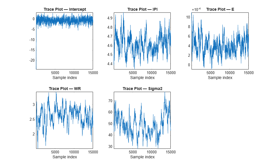
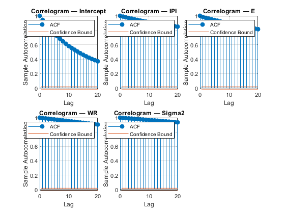
All parameters, except the intercept, show significant transient effects and high autocorrelation. estimate checks for high correlation, and, if present, issues warnings. Also, the parameters do not seem to have converged to their stationary distribution.
Estimate the posterior distribution again. To reduce transient effects, use the default burn-in period (5000, which is the default). To reduce the affects of serial correlation, thin by a factor of 20 and specify 15e4/thin effective number of draws. Also, numerically stabilize the estimation of by specifying reparameterize to  . Plot trace and autocorrelation plots.
thin = 20;
numDraws = 15e4/thin;
PosteriorMdl2 = estimate(PriorMdl,X,y,'Thin',thin,'Width',width,...
    'Reparameterize',true,'NumDraws',numDraws);

figure;
for j = 1:4
    subplot(2,3,j)
    plot(PosteriorMdl2.BetaDraws(j,:));
    axis tight
    xlabel('Sample index')
    title(sprintf(['Trace Plot ' char(8212) '%s'],PriorMdl.VarNames{j}));
end
subplot(2,3,5)
plot(PosteriorMdl2.Sigma2Draws);
axis tight
xlabel('Sample index')
title(['Trace Plot ' char(8212) ' Sigma2']);

figure;
for j = 1:4
    subplot(2,3,j)
    autocorr(PosteriorMdl2.BetaDraws(j,:));
    title(sprintf(['Correlogram ' char(8212) ' %s'],PriorMdl.VarNames{j}));
end
subplot(2,3,5)
autocorr(PosteriorMdl2.Sigma2Draws);
title(['Correlogram  ' char(8212) ' Sigma2']);
Method: MCMC sampling with 7500 draws
Number of observations: 62
Number of predictors:   4

           |   Mean     Std         CI95        Positive  Distribution
-----------------------------------------------------------------------
 Intercept | -0.4777  1.2225  [-2.911,  1.955]    0.338     Empirical
 IPI       |  4.6506  0.1128  [ 4.434,  4.884]    1.000     Empirical
 E         |  0.0005  0.0002  [ 0.000,  0.001]    0.991     Empirical
 WR        |  2.5243  0.3468  [ 1.815,  3.208]    1.000     Empirical
 Sigma2    | 51.3444  9.3170  [36.319, 72.469]    1.000     Empirical
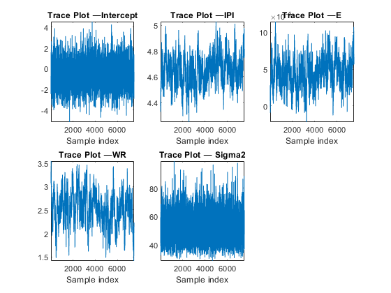
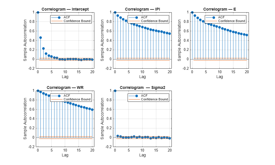
The trace plots suggest that the Markov chains:
Have reached their stationary distributions because the distribution of the samples have a relatively constant mean and variance. Specifically, the distribution of the points does not seem to change.
Are mixing fairly quickly because the serial correlation is moderate, for some parameters, to very low.
Do not show any transient behavior.
These results suggest that you can proceed with a sensitivity analysis, or with posterior inference.