Develop Fixed-Point Algorithms

This example shows how to develop and verify a simple fixed-point algorithm. This example follows these steps for algorithm development:

1) Implement a second-order filter algorithm and simulate in double-precision floating-point.

2) Instrument the code to visualize the dynamic range of the output and state.

3) Convert the algorithm to fixed point by changing the data type of the variables. The algorithm itself does not change.

4) Compare and plot the fixed-point and floating-point results.

Define Double-Precision Floating-Point Variables

Develop the algorithm in double-precision floating-point. The algorithm used in this example is a second-order lowpass filter that removes the high frequencies in the input signal.

Define numerator coefficients, a, and denominator coefficients, b.

b = [ 0.25 0.5      0.25    ];
a = [ 1    0.09375  0.28125 ];

Generate a random input that has both high and low frequencies.

s = rng; rng(0,'v5uniform');
x = randn(1000,1);
rng(s); % restore |rng| state

Pre-allocate the output, y, and state, z, for speed.

y = zeros(size(x));
z = [0;0];

Implement Data Type Independent Algorithm

This is a second-order filter that implements the standard difference equation:

|y(n) = b(1)*x(n) + b(2)*x(n-1) + b(3)*x(n-2) - a(2)*y(n-1) - a(3)*y(n-2)|

for k=1:length(x)
    y(k) =  b(1)*x(k) + z(1);
    z(1) = (b(2)*x(k) + z(2)) - a(2)*y(k);
    z(2) =  b(3)*x(k)         - a(3)*y(k);
end

Save the floating-point result.

ydouble = y;

Instrument Floating-Point Code to Visualize Dynamic Range

To convert to fixed point, we need to know the range of the variables. Depending on the complexity of an algorithm, this task can be simple or quite challenging. In this example, the range of the input value is known, so selecting an appropriate fixed-point data type is simple. Concentrate on the output (y) and states (z) since their range is unknown. To view the dynamic range of the output and states, modify the code slightly to instrument it.

Create a NumericTypeScope object and view the dynamic range of states (z).

z = [0;0]; % Reset states

hscope1 = NumericTypeScope;

for k=1:length(x)
    y(k) =  b(1)*x(k) + z(1);
    z(1) = (b(2)*x(k) + z(2)) - a(2)*y(k);
    z(2) =  b(3)*x(k)         - a(3)*y(k);

    % Process the data and update the visual
    step(hscope1,z);
end

% Clear the information stored in the object hscope1
reset(hscope1);

Create a NumericTypeScope object and view the dynamic range of the output y.

hscope2 = NumericTypeScope;

step(hscope2,y);

% Clear the information stored in the object hscope2
reset(hscope2);

First, analyze the information displayed for variable z (state). From the histogram, observe that the dynamic range lies within [(2^(1) 2^(-12)]. By default, the scope uses a data type of numerictype('double'). You can adjust the Proposed Data Type field in the scope to see that a data type of numerictype(true,16,14) results in zero overflows.

Next, look at variable y (output). From the histogram plot we see that the dynamic range lies within [(2^(1) 2^(-13)]. Again, a data type of numerictype(true,16,14) reports zero overflows or underflows in the scope.

Define Fixed-Point Variables

Convert variables to use fixed-point data types and run the algorithm again.

Enable logging to see the overflows and underflows introduced by the selected data types.

FIPREF_STATE = get(fipref);
reset(fipref)
fp = fipref;
default_loggingmode = fp.LoggingMode;
fp.LoggingMode = 'On';

Capture the present state of and reset the global fimath to the factory settings.

globalFimathAtStart = fimath;
resetglobalfimath;

Define the fixed-point types for the variables in the below format: fi(Data, Signed, WordLength, FractionLength)

b = fi(b, 1, 8, 6);
a = fi(a, 1, 8, 6);

x = fi(x, 1, 16, 13);
y = fi(zeros(size(x)), 1, 16, 13);
z = fi([0;0], 1, 16, 14);

Implement the Same Data Type Independent Algorithm

for k=1:length(x)
    y(k) =  b(1)*x(k) + z(1);
    z(1) = (b(2)*x(k) + z(2)) - a(2)*y(k);
    z(2) =  b(3)*x(k)         - a(3)*y(k);
end
% Reset the logging mode.
fp.LoggingMode = default_loggingmode;

In this example, we have redefined the fixed-point variables with the same names as the floating-point so that we could inline the algorithm code for clarity. However, it is a better practice to enclose the algorithm code in a MATLAB® file function that could be called with either floating-point or fixed-point variables.

Compare and Plot the Floating-Point and Fixed-Point Results

Plot the magnitude response of the floating-point and fixed-point results and the response of the filter to see if the filter behaves as expected when it is converted to fixed-point.

n = length(x);
f = linspace(0,0.5,n/2);
x_response = 20*log10(abs(fft(double(x))));
ydouble_response = 20*log10(abs(fft(ydouble)));
y_response = 20*log10(abs(fft(double(y))));
plot(f,x_response(1:n/2),'c-',...
    f,ydouble_response(1:n/2),'bo-',...
    f,y_response(1:n/2),'gs-');
ylabel('Magnitude in dB');
xlabel('Normalized Frequency');
legend('Input','Floating point output','Fixed point output','Location','Best');
title('Magnitude response of Floating-point and Fixed-point results');

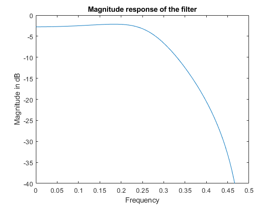
h = fft(double(b),n)./fft(double(a),n); 
h = h(1:end/2);
clf
hax = axes;
plot(hax,f,20*log10(abs(h)));
set(hax,'YLim',[-40 0]);
title('Magnitude response of the filter');
ylabel('Magnitude in dB')
xlabel('Frequency');

Notice that the high frequencies in the input signal are attenuated by the low-pass filter which is the expected behavior.

Plot the Error

clf
n = (0:length(y)-1)';
e = double(lsb(y));
plot(n,double(y)-ydouble,'.-r', ...
     [n(1) n(end)],[e/2 e/2],'c', ...
     [n(1) n(end)],[-e/2 -e/2],'c')
text(n(end),e/2,'+1/2 LSB','HorizontalAlignment','right','VerticalAlignment','bottom')
text(n(end),-e/2,'-1/2 LSB','HorizontalAlignment','right','VerticalAlignment','top')
xlabel('n (samples)'); ylabel('error')

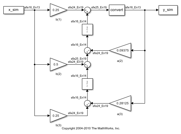
Implement the Algorithm in Simulink

If you have Simulink® and Fixed-Point Designer™, you can run the fitdf2filter_demo model, which is the equivalent of the algorithm above. The output, y_sim is a fixed-point variable equal to the variable y calculated above in MATLAB® code.

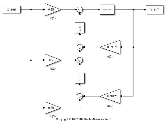
As in the MATLAB code, the fixed-point parameters in the blocks can be modified to match an actual system. These have been set to match the MATLAB code in the example above. Double-click the blocks to see the settings.

% Set up the From Workspace variable
x_sim.time = n;
x_sim.signals.values = x;
x_sim.signals.dimensions = 1;

% Run the simulation
out_sim = sim('fitdf2filter_demo', 'SaveOutput', 'on', ...
    'SrcWorkspace', 'current');
    
% Open the model
open_system('fitdf2filter_demo')
    
% Verify that the Simulink results are the same as the MATLAB file
isequal(y, out_sim.get('y_sim'))

ans = logical
   1

Assumptions Made for This Example

In order to simplify the example, these default math parameters were used: round-to-nearest, saturate on overflow, full precision products and sums. You can modify all of these parameters to match an actual system.

The settings were chosen as a starting point in algorithm development. Save a copy of this MATLAB file, start playing with the parameters, and see what effects they have on the output. How does the algorithm behave with a different input? See the help for fi, fimath, and numerictype for information on how to set other parameters, such as rounding mode, and overflow mode.

% Reset the global fimath
globalfimath(globalFimathAtStart);
fipref(FIPREF_STATE);