Representar el frente de Pareto en 3D
Este ejemplo muestra cómo representar un frente de Pareto para tres objetivos. Cada función objetivo es el cuadrado de la distancia desde un punto 3D particular. Para acelerar el cálculo, escriba cada función objetivo en forma vectorizada como un producto escalar. Para obtener un conjunto de soluciones denso, utilice 200 puntos en el frente de Pareto.
El ejemplo muestra primero cómo obtener el gráfico utilizando la función de gráfico incorporada 'psplotparetof'. Luego resuelva el mismo problema y obtenga la gráfica usando gamultiobj, lo que requiere configuraciones de opciones ligeramente diferentes. El ejemplo muestra cómo obtener variables de solución para un punto particular en el diagrama de Pareto. Luego, el ejemplo muestra cómo representar los puntos directamente, sin utilizar una función de representación, y muestra cómo representar una superficie interpolada en lugar de puntos de Pareto.
fun = @(x)[dot(x - [1,2,3],x - [1,2,3],2), ...
    dot(x - [-1,3,-2],x - [-1,3,-2],2), ...
    dot(x - [0,-1,1],x - [0,-1,1],2)];
options = optimoptions('paretosearch','UseVectorized',true,'ParetoSetSize',200,...
    'PlotFcn','psplotparetof');
lb = -5*ones(1,3);
ub = -lb;
rng default % For reproducibility
[x,f] = paretosearch(fun,3,[],[],[],[],lb,ub,[],options);
Pareto set found that satisfies the constraints.

Optimization completed because the relative change in the volume of the Pareto set
is less than 'options.ParetoSetChangeTolerance' and constraints are satisfied to within
'options.ConstraintTolerance'.
opts = optimoptions('gamultiobj',"PlotFcn","gaplotpareto","PopulationSize",200);
[xg,fg] = gamultiobj(fun,3,[],[],[],[],lb,ub,[],opts);
gamultiobj stopped because the average change in the spread of Pareto solutions is less than options.FunctionTolerance.
Este gráfico muestra muchos menos puntos que el gráfico paretosearch. Resuelva el problema nuevamente utilizando una población más grande.
opts.PopulationSize = 400;
[xg,fg] = gamultiobj(fun,3,[],[],[],[],lb,ub,[],opts);
gamultiobj stopped because the average change in the spread of Pareto solutions is less than options.FunctionTolerance.
Cambie el ángulo de visión para que coincida mejor con el gráfico psplotpareto.
view(-40,57)
Encontrar el punto de solución utilizando sugerencias de herramientas
Seleccione un punto en el gráfico utilizando la herramienta Data Tips.
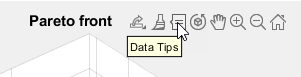
El punto ilustrado tiene índice 92. Muestra el punto xg(92,:) que contiene las variables de solución asociadas con el punto representado.
disp(xg(92,:))
-0.2889 0.0939 0.4980
Evalúe las funciones objetivo en este punto para ver que coincidan con los valores mostrados.
disp(fun(xg(92,:)))
11.5544 15.1912 1.5321
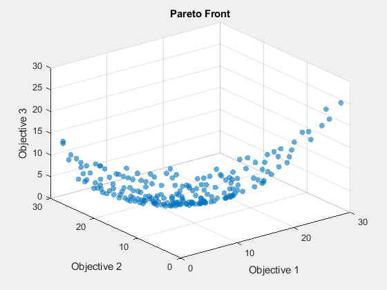
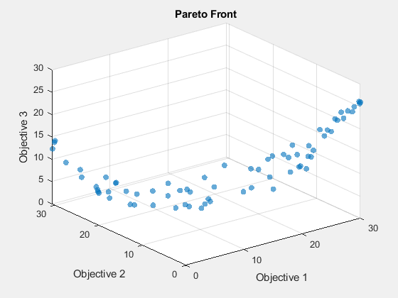
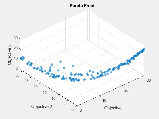
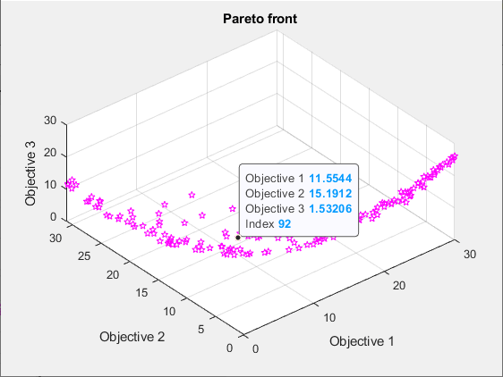
Crear un diagrama de dispersión en 3D
Grafique puntos en el frente de Pareto utilizando scatter3 .
figure
subplot(2,2,1)
scatter3(f(:,1),f(:,2),f(:,3),'k.');
subplot(2,2,2)
scatter3(f(:,1),f(:,2),f(:,3),'k.');
view(-148,8)
subplot(2,2,3)
scatter3(f(:,1),f(:,2),f(:,3),'k.');
view(-180,8)
subplot(2,2,4)
scatter3(f(:,1),f(:,2),f(:,3),'k.');
view(-300,8)
Al girar la gráfica de forma interactiva, obtendrás una mejor visión de su estructura.
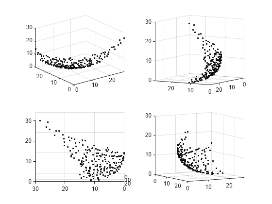
Gráfica de superficie interpolada
Para ver el frente de Pareto como una superficie, cree un interpolante disperso.
figure
F = scatteredInterpolant(f(:,1),f(:,2),f(:,3),'linear','none');
Para representar la superficie resultante, cree una malla en el espacio x-y desde los valores más pequeños hasta los más grandes. A continuación, represente la superficie interpolada.
sgr = linspace(min(f(:,1)),max(f(:,1)));
ygr = linspace(min(f(:,2)),max(f(:,2)));
[XX,YY] = meshgrid(sgr,ygr);
ZZ = F(XX,YY);
Grafique los puntos de Pareto y la superficie juntos.
figure
subplot(2,2,1)
surf(XX,YY,ZZ,'LineStyle','none')
hold on
scatter3(f(:,1),f(:,2),f(:,3),'k.');
hold off
subplot(2,2,2)
surf(XX,YY,ZZ,'LineStyle','none')
hold on
scatter3(f(:,1),f(:,2),f(:,3),'k.');
hold off
view(-148,8)
subplot(2,2,3)
surf(XX,YY,ZZ,'LineStyle','none')
hold on
scatter3(f(:,1),f(:,2),f(:,3),'k.');
hold off
view(-180,8)
subplot(2,2,4)
surf(XX,YY,ZZ,'LineStyle','none')
hold on
scatter3(f(:,1),f(:,2),f(:,3),'k.');
hold off
view(-300,8)
Al girar la gráfica de forma interactiva, obtendrás una mejor visión de su estructura.
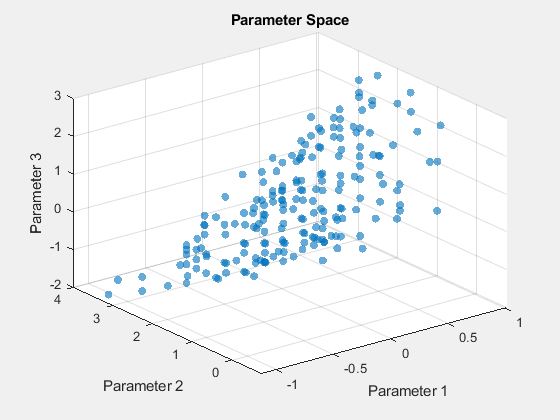
Representar el conjunto de Pareto en el espacio de variables de control
Puede obtener un gráfico de los puntos del conjunto de Pareto utilizando la función de gráfico 'psplotparetox'.
options.PlotFcn = 'psplotparetox';
[x,f] = paretosearch(fun,3,[],[],[],[],lb,ub,[],options);
Pareto set found that satisfies the constraints. Optimization completed because the relative change in the volume of the Pareto set is less than 'options.ParetoSetChangeTolerance' and constraints are satisfied to within 'options.ConstraintTolerance'.
Alternativamente, cree un diagrama de dispersión de los valores x en el conjunto de Pareto.
figure
subplot(2,2,1)
scatter3(x(:,1),x(:,2),x(:,3),'k.');
subplot(2,2,2)
scatter3(x(:,1),x(:,2),x(:,3),'k.');
view(-148,8)
subplot(2,2,3)
scatter3(x(:,1),x(:,2),x(:,3),'k.');
view(-180,8)
subplot(2,2,4)
scatter3(x(:,1),x(:,2),x(:,3),'k.');
view(-300,8)
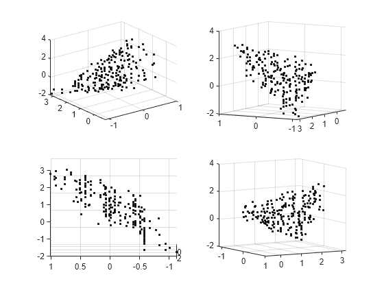
Este conjunto no tiene una superficie transparente. Al girar la gráfica de forma interactiva, obtendrás una mejor visión de su estructura.
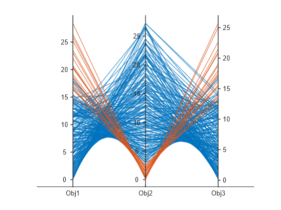
Gráfica paralela
Puedes representar gráficamente el conjunto de Pareto utilizando un gráfico de coordenadas paralelas. Puede utilizar un gráfico de coordenadas paralelas para cualquier número de dimensiones. En el gráfico, cada línea coloreada representa un punto de Pareto y cada variable de coordenadas corresponde a una línea vertical asociada. Grafique los valores de la función objetivo utilizando parellelplot .
figure
p = parallelplot(f);
p.CoordinateTickLabels =["Obj1";"Obj2";"Obj3"];
Colorea los puntos de Pareto en la décima más baja de los valores de Obj2 .
minObj2 = min(f(:,2));
maxObj2 = max(f(:,2));
grpRng = minObj2 + 0.1*(maxObj2-minObj2);
grpData = f(:,2) <= grpRng;
p.GroupData = grpData;
p.LegendVisible = "off";