Single-Stage Primary Cylinder
R2026bThis example shows how to model, parameterize, and test a single-stage primary cylinder, starting from manufacturer data sheet information. In this example, you calculate the unknown parameters given the numerical data extracted from the data sheet. After you simulate the model, you can compare the simulation push rod force versus pressure relationship curve with curve provided on the manufacturer data sheet.
Open the Model
The SingleStagePrimaryCylinder model, which is a model of a single-stage primary cylinder with a test harness.
open_system('SingleStagePrimaryCylinder')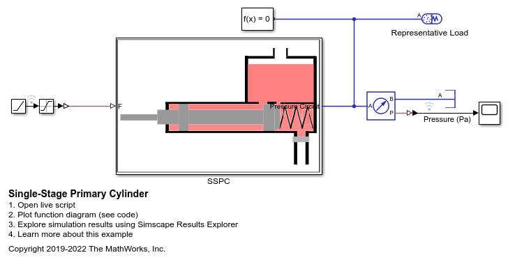
Manufacturer Data Sheet Data
Define data for the supplier component design parameters and the expected output function diagram.
sspc.dp = 31.75*1e-3;               % (m) Piston diameter
sspc.stroke = 36*1e-3;              % (m) Piston stroke
sspc.disp = 27*1e-6;                % (m^3) Circuit displacement
sspc.maxPress = 120*1e5;            % (Pa or N/m^2) Max pressure

sspc.pushRodF = [0 100 4000];       % (N) Push rod force
sspc.circuitP = [0 0   45e5];       % (Pa or N/m^2) Pressure vector
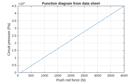
Plot the function diagram of single-stage primary cylinder.
p1 = plot(sspc.pushRodF,sspc.circuitP);
p2 = xlabel('Push rod force (N)');
p3 = ylabel('Circuit pressure (Pa)');
p4 = title('Function diagram from data sheet');
grid on
Calculate derived parameters or make assumptions for the remaining parameters.
sspc.aPist = (pi/4)*sspc.dp^2;                              % (m^2) Pressure acting piston area
sspc.deadzone = 1.5e-3;                                     % (m) length for which no pressure generated
sspc.c = 1e-3;                                              % (Ns/m) Damping coefficient
sspc.mass = 1e-2;                                           % (Kg) Piston mass
sspc.v2D = 1000e-9;                                         % (m^3) Circuit dead Volume
sspc.v2M = sspc.v2D+sspc.aPist*(sspc.stroke-sspc.deadzone); % (m^3) Circuit max Volume
sspc.a1Ori = 100e-6;                                        % (m^2) Compensating orifice area
sspc.a2Ori = 10e-6;                                         % (m^2) Circuit orifice area
sspc.pRes = 1e5;                                            % (Pa) Initial Pressure condition
sspc.hss = 1e8;                                             % (N/m) Hard stop stiffness
sspc.hsd = 1e6;                                             % (N/(m/s)) Hard stop damping coefficient
Parameter Estimation Scheme
The equation of motion of the single-stage primary cylinder system is
The steady-state equation of the system is
where:
is positions of mass from the left side assumed hard stop.
is mass of piston.
is damping coefficient of piston.
is spring stiffness coefficients.
is force applied on push rod of primary cylinder.
is pressures in brake circuit.
is preload on the spring.
You can solve the steady-state equation of the system at the two points given in the function diagram. Use the solution as parameters that govern the functionality of the system.
sspc.fP1 = sspc.pushRodF(2);
sspc.fP2 = sspc.pushRodF(3);
sspc.P1 = sspc.circuitP(2);
sspc.P2 = sspc.circuitP(3);
sspc.a = [sspc.deadzone 1; ...
         sspc.stroke   1];
sspc.b = [sspc.fP1 - sspc.P1*sspc.aPist; ...
         sspc.fP2 - sspc.P2*sspc.aPist];
sspc.out = sspc.a\sspc.b;

sspc.k = sspc.out(1);              % (N/m) Spring stiffness
sspc.preL = sspc.out(2);           % (N) Spring preload force
sspc.def = sspc.preL/sspc.k;       % (m) Spring compression
Set Model Up for Simulation
It is important to test the system with the correct load. In the test model, a spring-based accumulator performs the loading on the single-stage primary cylinder. Use information from the data sheet to determine the stroke values for circuits.
sspc.vol = sspc.v2M-sspc.v2D-sspc.aPist*sspc.deadzone;   % (m^3) Fluid chamber capacity for pressure circuit
sspc.loadP = sspc.circuitP(3);                           % (Pa) Pressure at full capacity for pressure circuit
Simulate the Model
The model generates push rod force versus pressure plots for selected manufacturer designs. The applied push rod force to the single-stage primary cylinder is ramped at 25 N/sec in the simulation.
 simT = (sspc.pushRodF(3)/25)+10; % Simulation time
 sim('SingleStagePrimaryCylinder.slx',simT)
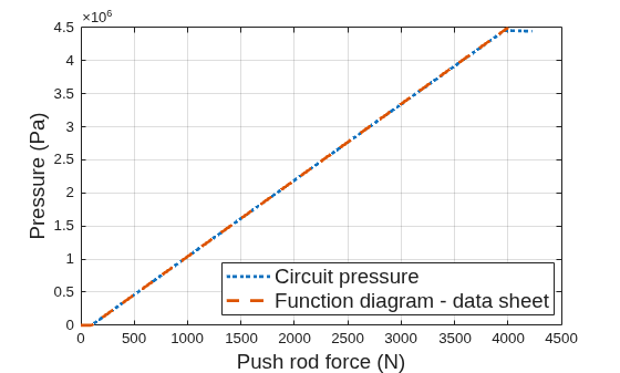
Plot the output from the model and the results with the data sheet functional specification. The plot shows that the results match, which means that you parameterized the block correctly.
figure
i1 = plot(logsout{1}.Values.Time,...
    logsout{2}.Values.Data);
i2 = xlabel('Time (sec)');
i3 = ylabel('Push rod force (N)');
i4 = title('Model force applied by driver on push rod');
i1.LineWidth = 2;
i2.FontSize = 14;
i3.FontSize = 14;
i4.FontSize = 14;
grid on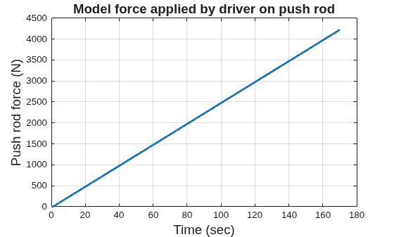
figure
p5 = plot(logsout{2}.Values.Data,logsout{1}.Values.Data,...
    ':',sspc.pushRodF,sspc.circuitP,'--');
p6 = legend('Circuit pressure','Function diagram - data sheet','location','best');
grid on
p5(1).LineWidth = 2;
p5(2).LineWidth = 2;
p7 = xlabel('Push rod force (N)');
p8 = ylabel('Pressure (Pa)');
p6.FontSize = 14;
p7.FontSize = 14;
p8.FontSize = 14;