Estimate Nonlinear Autonomous Neural State-Space System Using Mini-Batch Learning

This example shows how to use the mini-batch learning mode to estimate a nonlinear neural state-space model with no inputs and a two-dimensional continuous state equal to the output. First, you collect identification and validation data by simulating a Van der Pol system, and then you use the collected data to estimate and validate a neural state-space system.

Define Model for Data Collection

Define a time-invariant continuous-time autonomous model that you can easily simulate to collect data. For this example, use an unforced Van der Pol oscillator (VDP) system, which is an oscillator with nonlinear damping that exhibits a limit cycle.

Specify the state equation using an anonymous function, using a damping coefficient of 1.

dx = @(x) [x(2); 1*(1-x(1)^2)*x(2)-x(1)];

Generate Data Set for Training

Fix the random generator seed for reproducibility.

rng default

Run 1000 simulations each starting at a different initial state and lasting two seconds. Each experiment must use identical time points. Use a sampling rate of 0.01 seconds and add noise to make the data set more challenging.

N = 1000;
t = (0:0.01:2)';
Y = cell(1,N);

for i = 1:N
   % Create random initial state within [-2,2]
   x0 = 4*rand(2,1)-2;

   % Obtain state measurements over t (solve using ode45)
   [~, x] = ode45(@(t,x) dx(x),t,x0);

   % Add noise to make dataset more challenging
   x = x + 0.05*randn(size(t));

   % Each experiment in the data set is a timetable
   Y{i} = array2timetable(x,RowTimes=seconds(t));
end

Generate Data Set for Validation

Run one simulation to collect data that you will use to visually inspect the training result during the identification progress. The validation data set can have different time points. For this example, use the trained model to predict VDP behavior for 10 seconds.

% Create random initial state within [-2,2]
t = (0:0.1:10)';
x0 = 4*rand(2,1)-2;

% Obtain state measurements over t (solve using ode45)
[~, x] = ode45(@(t,x) dx(x),t,x0);

% Append the validation experiment (also a timetable) as the last entry in the data set
Y{end+1} = array2timetable(x,RowTimes=seconds(t));

Create Neural State-Space Object

Create a time-invariant continuous-time neural state-space object with a two-element state vector identical to the output, and no input.

nss = idNeuralStateSpace(2);

Configure State Network

Define the neural network that approximates the state function as having two hidden layers with 12 neurons each, and a hyperbolic tangent activation function.

Use createMLPNetwork to create the network and dot notation to assign it to the StateNetwork property of nss.

nss.StateNetwork = createMLPNetwork(nss,'state', ...
    LayerSizes=[12 12], ...
    Activations="tanh", ...
    WeightsInitializer="glorot", ...
    BiasInitializer="zeros");

Display the number of network parameters.

summary(nss.StateNetwork)

   Initialized: true

   Number of learnables: 218

   Inputs:
      1   'x'   2 features

Specify the training options for the state network using nssTrainingOptions. Use the Adam algorithm and specify the maximum number of epochs as 90. An epoch is the full pass of the training algorithm over the entire training set.

opt = nssTrainingOptions('adam');
opt.MaxEpochs = 90;

To speed up training, split the data set into smaller windows of size 20 each using the WindowSize property. Based on practical experience, segmentation usually improves the estimation performance.

opt.WindowSize = 20;

To enable mini-batch learning, set the NumWindowFraction property. For this example, specify NumWindowFraction as 0.2. In each iteration, the software uses only 20% of the windows to update the network parameters. Consequently, each epoch consists of five (1/0.2) iterations, which means that the software updates the network parameters five times per epoch.

opt.NumWindowFraction = 0.2;

Specify the learning rate.

opt.LearnRate = 0.04;

Estimate Neural State-Space System

To train the state network of nss using the identification data set and the predefined set of optimization options, use nlssest. Return the optimal model parameters during training using the params output argument.

[nss,params] = nlssest([],Y,nss,opt,'UseLastExperimentForValidation',true,'ValidationFrequency',10);

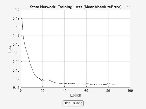
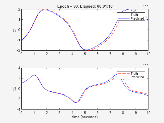
Generating estimation report...done.

The validation plot shows that the resulting system is able to generalize well to the validation data.

Update Parameters of Neural State-Space System

Display the params output argument. It contains the loss and network parameters corresponding to the final model, the model with minimal training loss, and the model with minimal validation loss.

params

params=3×4 table
            Type            TrainingLoss    ValidationLoss      Parameters  
    ____________________    ____________    ______________    ______________

    "Final_Loss"              0.11304           0.18444       {218×1 double}
    "MinTraining_Loss"        0.11304           0.18444       {218×1 double}
    "MinValidation_Loss"      0.11307          0.089952       {218×1 double}

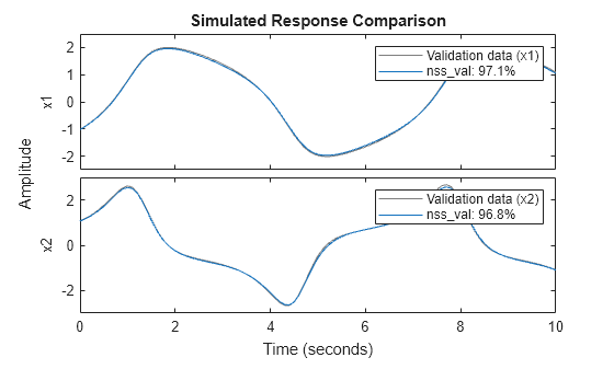
To update the model and use the network parameters corresponding to the model with minimal validation loss, use the setpvec command.

nss_val = setpvec(nss,params.Parameters{3});

Plot the response of both the estimated model and the updated model over the validation data set. You can see that nss_val performs much better on the validation data set.

Y_validation = Y{end};
compare(Y_validation,nss)
compare(Y_validation,nss_val)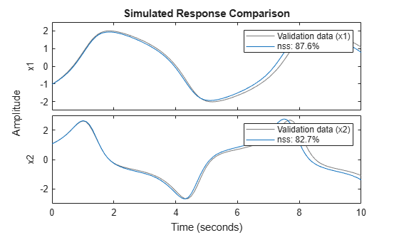

legend(Interpreter="none")