Display Vector Data as Lines and Patches
Display vector data on maps as lines and patches (filled polygons).
This page shows how to create similar maps using map axes (since R2023a) and axesm-based maps. For a comparison of map axes and axesm-based maps, including when to use each type of display, see Choose a 2-D Map Display.
Prepare Data
Prepare the data to use in the examples.
Read a shapefile of US states into a geospatial table. The table represents the states using polygon shapes in geographic coordinates. Create a subtable of states in the conterminous US.
statesGT = readgeotable("usastatehi.shp");

rows = statesGT.Name ~= "Hawaii" & statesGT.Name ~= "Alaska";
conusGT = statesGT(rows,:);
Read a shapefile of world rivers into a geospatial table. The table represents the rivers using line shapes in geographic coordinates. Clip the rivers to the geographic limits of the conterminous US.
riversGT = readgeotable("worldrivers.shp");

[latlim,lonlim] = bounds(conusGT.Shape,"all");
clippedRivers = geoclip(riversGT.Shape,latlim,lonlim);
riversGT.Shape = clippedRivers;
Read a shapefile of world lakes into a geospatial table. Create a subtable that contains the Great Lakes.
lakesGT = readgeotable("worldlakes.shp");

lakeNames = ["Lakes Superior, Michigan, Huron","Lake Ontario","Lake Erie"];
greatLakesGT = geocode(lakeNames,lakesGT);
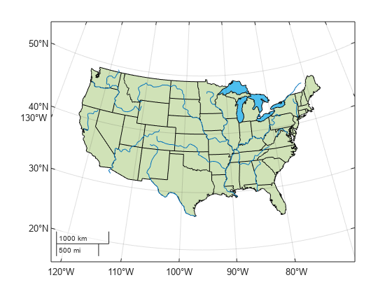
Create Map Using Map Axes
Display vector data on a map axes object using lines and polygons.
Set up a map using a projected coordinate reference system (CRS) that is appropriate for the conterminous United States. Create the projected CRS using the ESRI code 102003.
figure
proj = projcrs(102003,Authority="ESRI");
newmap(proj)
hold on
Display the data on the map by using the geoplot function.
Display the states using green polygons.
Display the Great Lakes using opaque, light blue polygons.
Display the rivers using blue lines.
geoplot(statesGT,FaceColor=[0.4660 0.6740 0.1880])
geoplot(greatLakesGT,FaceAlpha=1,FaceColor=[0.3010 0.7450 0.9330])
geoplot(riversGT,Color=[0 0.4470 0.7410])
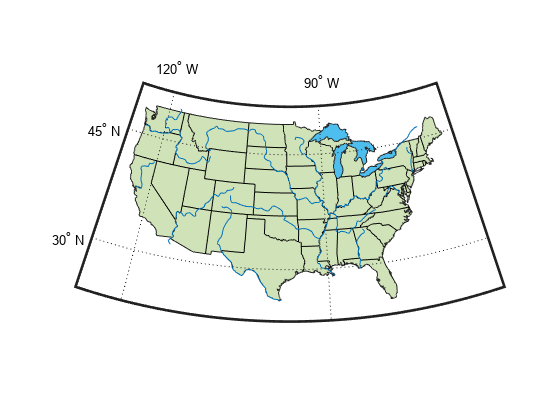
Create Map Using axesm-Based Map
Display vector data on an axesm-based map using lines and patches.
Create a polygon shape that extends outside of the conterminous US by using the union and buffer functions. Then, calculate the latitude and longitude limits to use for the axesm-based map by using the bounds function.
statesUnion = union(conusGT.Shape);
buffered = buffer(statesUnion,2);
[latlim,lonlim] = bounds(buffered);
Create an axesm-based map by using the axesm function, an Equal Area Conic projection, and the calculated limits. When you specify map limits, the map automatically centers the projection on an appropriate longitude. Use the default latitudes for the standard parallels by specifying the MapParallels argument as an empty matrix.
figure
axesm(MapProjection="eqaconic",MapParallels=[], ...
    MapLatLimit=latlim,MapLonLimit=lonlim)
axis off
Display the map frame, map grid, meridian labels, and parallel labels.
framem
gridm
mlabel
plabel
Display the data on the map by using the geoshow function.
Display the states using green patches.
Display the Great Lakes using light blue patches.
Display the rivers using blue lines.
geoshow(conusGT,FaceColor=[0.8157 0.8863 0.7176])
geoshow(greatLakesGT,FaceColor=[0.3010 0.7450 0.9330])
geoshow(riversGT,Color=[0 0.4470 0.7410])
Tips
Unlike the
axesmfunction, theworldmapandusamapfunctions automatically select appropriate limits based on the input data.To plot data that is already in projected coordinates, use a regular axes object and the
mapshowfunction.