Geolocated Data Grids
In addition to regular data grids, the toolbox provides another format for geodata: geolocated data grids. These multivariate data sets can be displayed, and their values and coordinates can be queried, but unfortunately much of the functionality supporting regular data grids is not available for geolocated data grids.
Regular data grids cover simple, regular quadrangles, that is, geographically rectangular and aligned with parallels and meridians. Geolocated data grids, in addition to these rectangular orientations, can have other shapes as well.
Define Geolocated Data Grid
To define a geolocated data grid, you must define three variables: a matrix of indices or values associated with the mapped region, a matrix giving cell-by-cell latitude coordinates, and a matrix giving cell-by-cell longitude coordinates.
Load a MAT-file containing an irregularly shaped geolocated data grid called mapmtx.
load mapmtxView the variables created from this MAT-file. Two geolocated data grids are in this data set, each requiring three variables. The values contained in map1 correspond to the latitude and longitude coordinates, respectively, in lt1 and lg1. Notice that all three matrices are the same size. Similarly, map2, lt2, and lg2 together form a second geolocated data grid. These data sets were extracted from the topo60c data grid. Neither of these maps is regular, because their columns do not run north to south.
whos
  Name              Size            Bytes  Class     Attributes

  description       1x54              108  char
  lg1              50x50            20000  double
  lg2              50x50            20000  double
  lt1              50x50            20000  double
  lt2              50x50            20000  double
  map1             50x50            20000  double
  map2             50x50            20000  double
  source            1x43               86  char
Display the grids one after another to see their geography.
close all
axesm mercator
gridm on
framem on
h1 = surfm(lt1,lg1,map1);
h2 = surfm(lt2,lg2,map2);

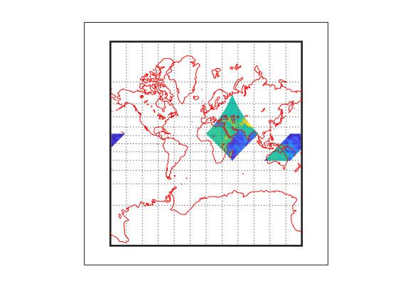
Showing coastlines will help to orient you to these skewed grids. Notice that neither grid is a regular rectangle. One looks like a diamond geographically, the other like a trapezoid. The trapezoid is displayed in two pieces because it crosses the edge of the map. These shapes can be thought of as the geographic organization of the data, just as rectangles are for regular data grids. But, just as for regular data grids, this organizational logic does not mean that displays of these maps are necessarily a specific shape.
load coastlines
plotm(coastlat,coastlon,'r')
Now change the view to a polyconic projection with an origin at 0°N, 90°E. As the polyconic projection is limited to a 150° range in longitude, those portions of the maps outside this region are automatically trimmed.
setm(gca,'MapProjection','polycon','Origin',[0 90 0])
