Create and Compare Resizing Interpolation Kernels
This example shows how to define a kernel for image resizing and compare different interpolation kernels on a sample image.
An interpolation kernel calculates the value of a pixel using a weighted average of neighboring pixel values. The imresize function offers many built-in kernels that perform bilinear, bicubic, and Lanczos resampling. You can also define a custom kernel and then resize images using the custom kernel.
To evaluate and compare interpolation kernels, this example magnifies a small image using each kernel. Fully assessing the performance of interpolation kernels requires examining a variety of different images and scale factors.
Create Kernels Based on imresize Interpolation Methods
The bilinear method uses a triangular interpolation kernel, which is defined as:
Create a bilinear interpolation kernel using a function called triangleResampling. This function is defined in the Helper Functions section at the end of this example. Then, display the bilinear interpolation kernel for a neighborhood of [-3.5, 3.5].
nhood = [-3.5 3.5];
fplot(@triangleResampling,nhood)
title("Bilinear (Triangular) Interpolation Kernel")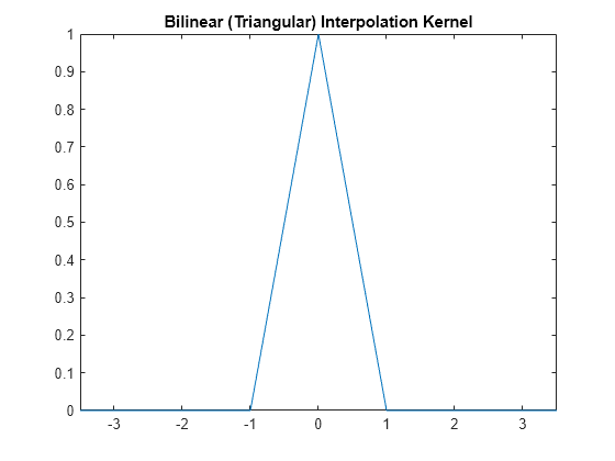
The bicubic method uses this piecewise cubic interpolation kernel:
Create a bicubic interpolation kernel using a helper function called bicubicResampling. This function is defined in the Helper Functions section at the end of this example. Then, display the bicubic interpolation kernel.
fplot(@bicubicResampling,nhood)
title("Bicubic Interpolation Kernel")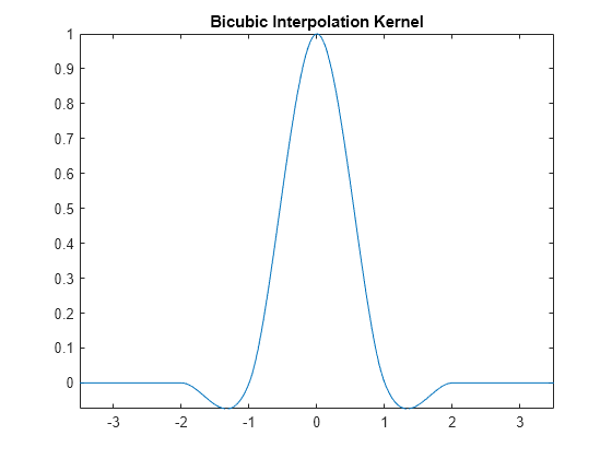
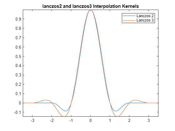
The lanczos2 and lanczos3 kernels are based on the Lanczos family of interpolation kernels. The Lanczos kernels are defined as follows, with or , respectively:
Create a lanczos2 and lanczos3 interpolation kernel using a function called lanczosResampling and specifying the factor .
lanczos2 = @(x) lanczosResampling(x,2);
lanczos3 = @(x) lanczosResampling(x,3);
Display the lanczos2 and lanczos3 interpolation kernels.
fplot(lanczos2,nhood)
hold on
fplot(lanczos3,nhood)
hold off
legend(["Lanczos 2","Lanczos 3"])
title("lanczos2 and lanczos3 Interpolation Kernels")
Define Custom Interpolation Kernel
Consider a piecewise rational function based on osculatory rational interpolation [1].
Create a custom interpolation kernel that performs osculatory rational interpolation using a function called oscResampling. This function is defined in the Helper Functions section at the end of this example. Then, display the custom interpolation kernel.
fplot(@oscResampling,nhood)
title("Custom Osculatory Rational Interpolation Kernel")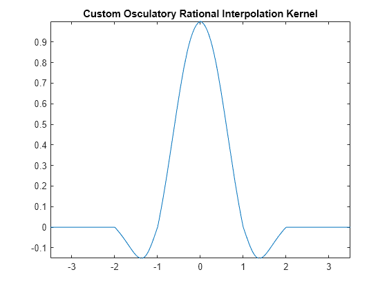
Resize Image Using Interpolation Kernels
Read and display a small icon image.
A = imread("region-analyzer-icon.png");Resize the image by a factor f using each built-in interpolation method. Note that the nearest-neighbor method does not take a weighted average of neighborhood pixels. Instead, the nearest neighbor method assigns the output pixels the value of the nearest input pixel.
f = 10;
B_nearest = imresize(A,f,'nearest');
B_bilinear = imresize(A,f,'bilinear');
B_bicubic = imresize(A,f,'bicubic');
B_lanczos2 = imresize(A,f,'lanczos2');
B_lanczos3 = imresize(A,f,'lanczos3');
To resize the image using the custom kernel, specify the function handle and the nonzero kernel width as the method argument for imresize:
width = 4;
B_osc = imresize(A,f,{@oscResampling,width});
Display the resized images as a tiled image, and compare the results subjectively.
The nearest-neighbor result (upper left) appears quite blocky. The bilinear result (upper center) is better in most respects than the nearest-neighbor result but looks a little blurry. The bicubic result (upper right) and lanczos2 result (lower left) appear very similar and are sharper than the bilinear result. For example, look closely at the digits "3" and "8" near the top of the image. The lanczos3 result (lower center) is sharper than the bicubic and lanczos2 results but exhibits a visible "ringing" artifact. The ringing artifact appears as a faint echo outside the gray boundary, or by looking just to the left and right of the thick black stripe running down the middle of the image.
The custom interpolation result (lower right) is slightly sharper than the bicubic and lanczos2 results with slightly smoother diagonal edges. The custom interpolation result does not exhibit a ringing artifact.
t = imtile({B_nearest,B_bilinear,B_bicubic, ...
    B_lanczos2,B_lanczos3,B_osc},BackgroundColor="white");
imshow(t)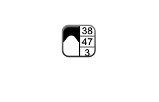
Helper Functions
The triangleResampling helper function performs bilinear interpolation.
function f = triangleResampling(x)
    f = (1 - abs(x)) .* (abs(x) <= 1);
end
The bicubicResampling helper function performs bicubic interpolation.
function f = bicubicResampling(x)
    absx = abs(x);
    absx2 = absx.^2;
    absx3 = absx.^3;

    f = (1.5*absx3 - 2.5*absx2 + 1) .* (absx <= 1) + ...
        (-0.5*absx3 + 2.5*absx2 - 4*absx + 2) .* ...
        ((1 < absx) & (absx <= 2));
end
The lanczosResampling helper function performs Lanczos interpolation using a specified factor a.
function f = lanczosResampling(x,a)
    f = a*sin(pi*x) .* sin(pi*x/a) ./ ...
        (pi^2 * x.^2);
    f(abs(x) > a) = 0;
    f(x == 0) = 1;
end
The oscResampling helper function performs osculatory rational interpolation.
function f = oscResampling(x)
    absx = abs(x);
    absx2 = absx.^2;

    f = (absx <= 1) .* ...
        ((-0.168*absx2 - 0.9129*absx + 1.0808) ./ ...
        (absx2 - 0.8319*absx + 1.0808)) ...
        + ...
        ((1 < absx) & (absx <= 2)) .* ...
        ((0.1953*absx2 - 0.5858*absx + 0.3905) ./ ...
        (absx2 - 2.4402*absx + 1.7676));
end
References
[1] Hu, Min, and Jieqing Tan. "Adaptive Osculatory Rational Interpolation for Image Processing." Journal of Computational and Applied Mathematics 195, no. 1–2 (October 2006): 46–53. https://doi.org/10.1016/j.cam.2005.07.011.