Interactively Fit Data and Visualize Model

The Basic Fitting tool lets you interactively model data for 2-D plots using a spline interpolant, a shape-preserving interpolant, or a polynomial up to the tenth degree. Using this tool, you can:

• Compute the model coefficients.

• Plot one or more models with the original data.

• Plot the residuals of the models.

• Compute the R-squared value and norm of residuals.

• Use the model to interpolate or extrapolate outside of the data.

• Save coefficients and computed values to the MATLAB workspace.

Load and Plot Data

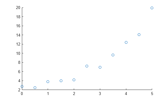
Create a sample predictor variable x and a sample response variable y. Visualize the data in a scatter plot.

If your data set is large and the values are not sorted in ascending order, the Basic Fitting tool takes more time to preprocess the data before fitting. You can speed up the Basic Fitting tool by first sorting the data.

x = [0:0.5:5]';
y = [2.73 2.50 3.79 3.98 4.21 7.18 6.95 9.63 12.39 14.10 19.93]';
scatter(x,y)

Fit Linear and Quadratic Models

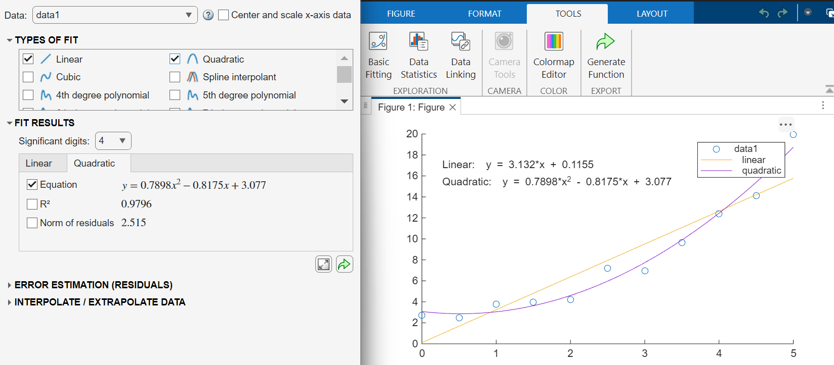
To use the Basic Fitting tool, on the Tools tab of the figure, click Basic Fitting. You can use the Basic Fitting tool to fit one or more models to the data. You can also use the tool to display the model and corresponding equations on the plot.

For example, fit a linear model and a quadratic model to the sample data. Select the Linear and Quadratic models in the Types of Fit section.

Validate Model

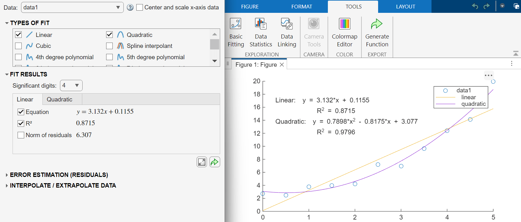
To validate a model, compute the coefficient of determination (R-squared). A value close to 1 indicates a good fit.

To display the R-squared value for a model on the plot, in the Fit Results section, select the tab for a model and select $R^2$. For example, display the R-squared value for the linear and quadratic models.

For higher-order models, a basic R-squared value does not fully account for the complexity of the model. A more appropriate measure for validating these models is the adjusted R-squared value. For more information, Linear Regression with One Predictor Variable.

Save Model Parameters to Workspace

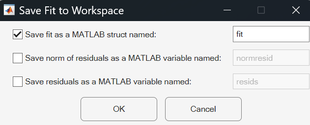
To access the model outside of the Basic Fitting tool, save the model data to the MATLAB workspace. Click the Export Results to Workspace button in the Fit Results section. In the Save Fit to Workspace dialog box that appears, select the parameters to save and click OK.

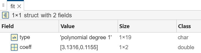
For example, save the model parameters for the linear model as a scalar structure fit.

The resulting structure contains two fields, type and coeff. You can use the coefficients to interpolate or extrapolate data. For example, evaluate the polynomial for the sample data points in xSample. You can view the contents of the structure in the Variables editor.

polyval(fit.coeff,xSample) 
openvar fit

You can access data in the structure by using dot notation. For example, access the vector of coefficients.

c = fit.coeff

Interpolate and Extrapolate Data

You can use a model to interpolate or extrapolate the data. In the Basic Fitting tool, in the Interpolate/Extrapolate Data section, enter a vector of query points. Then, you can display the data points on the plot by selecting Plot Evaluated Data. You can also export the data points to the MATLAB workspace by clicking the Export Evaluation to Workspace button.

For example, evaluate the quadratic model at query points [0.2 2.2 3.4]. Select the Quadratic tab in the Fit Results section. Then, in the Interpolate/Extrapolate Data section, enter the query point vector in the X field. A table with interpolated y values appears in the Basic Fitting tool. Add the interpolated values to the plot by selecting Plot evaluated data.

Fit New Data Using Generated Code

You can generate MATLAB code that recomputes fits and reproduces plots that you created using the Basic Fitting tool with new data.

In the figure window, on the Tools tab, click Generate Function . This creates a function named createfigure and displays it in the MATLAB Editor. The code programmatically reproduces what you did interactively with the Basic Fitting tool. Optionally rename the function, and save the code file.

Then, to recompute the models and reproduce the plots for new data, call the function and specify the new x- and y-data as the input arguments.

createfigure(xQuery,yQuery)