Design MPC Controller for Plant with Delays
This example shows how to design an MPC controller for a plant with delays using MPC Designer.
Plant Model
An example of a plant with delays is the distillation column model:
Outputs y1 and
y2 represent measured product purities. The
model consists of six transfer functions, one for each input/output pair. Each transfer
function is a first-order system with a delay. The longest delay in the model is
8.1 minutes.
Specify the individual transfer functions for each input/output pair. For example,
g12 is the transfer function from input
u2 to output
y1.
g11 = tf(12.8,[16.7 1],'IOdelay',1.0,'TimeUnit','minutes');
g12 = tf(-18.9,[21.0 1],'IOdelay',3.0,'TimeUnit','minutes');
g13 = tf(3.8,[14.9 1],'IOdelay',8.1,'TimeUnit','minutes');
g21 = tf(6.6,[10.9 1],'IOdelay',7.0,'TimeUnit','minutes');
g22 = tf(-19.4,[14.4 1],'IOdelay',3.0,'TimeUnit','minutes');
g23 = tf(4.9,[13.2 1],'IOdelay',3.4,'TimeUnit','minutes');
DC = [g11 g12 g13;
      g21 g22 g23];
Configure Input and Output Signals
Define the input and output signal names.
DC.InputName = {'Reflux Rate','Steam Rate','Feed Rate'};
DC.OutputName = {'Distillate Purity','Bottoms Purity'};
Alternatively, you can specify the signal names in MPC Designer, on the MPC Designer tab, by clicking I/O Attributes.
Specify the third input, the feed rate, as a measured disturbance (MD).
DC = setmpcsignals(DC,'MD',3);
Because they are not explicitly specified in setmpcsignals, all
other input signals are configured as manipulated variables (MV), and all output signals
are configured as measured outputs (MO) by default.
Open MPC Designer
Open MPC Designer importing the plant model.
mpcDesigner(DC)
Because DC is a stable, continuous-time LTI plant, MPC
Designer sets the controller sample time to 0.1 Tr, where Tr is the average rise
time of the plant. Because DC has a
Tr of is around 33 minutes, MPC
Designer sets a sample time of 3 minutes.
MPC Designer imports the specified plant to the Data Browser. The following objects are also created and added to the Data Browser:
mpc1— Default MPC controller created usingDCas its internal model.scenario1— Default simulation scenario.
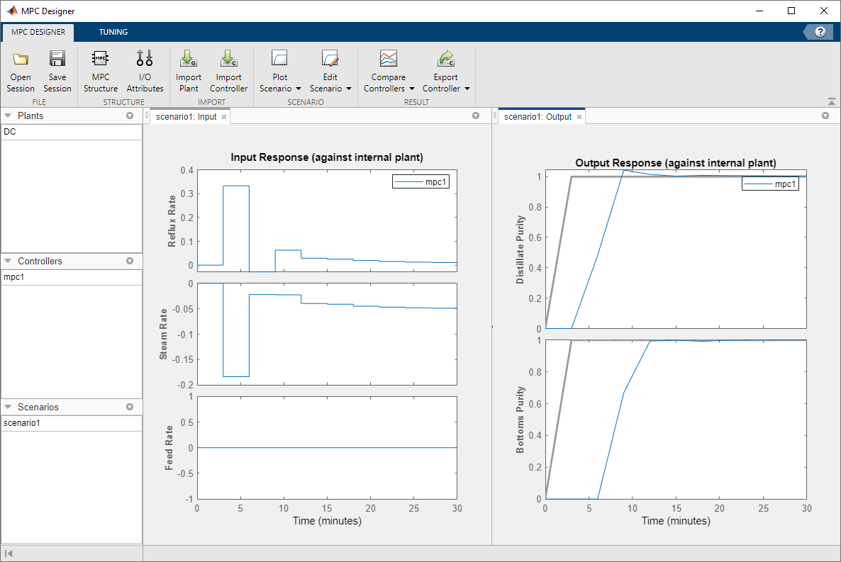
The app runs the simulation scenario and generates input and output response plots.
Specify Prediction and Control Horizons
For a plant with delays, it is good practice to specify the prediction and control horizons such that
where,
p is the prediction horizon.
m is the control horizon.
max(Td) is the maximum delay, which is
8.1minutes for theDCmodel.Δt is the controller Sample time, which is
3minutes for theDCmodel.
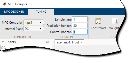
On the Tuning tab, in the Horizon section,
specify a Sample time of 1, a Prediction
horizon of 30, and a Control horizon
of 5.
After you change the horizons, the Input Response and Output Response plots for the default simulation scenario are automatically updated.
Simulate Controller Step Responses
On the MPC Designer tab, in the Scenario
section, click Edit Scenario > scenario1. Alternatively, in the Data Browser, right-click
scenario1 and select Edit.
In the Simulation Scenario dialog box, specify a Simulation
duration of 50 minutes.
In the Reference Signals table, in the
Signal drop-down list, select Step for
both outputs to simulate step changes in their setpoints.
Specify a step Time of 0 for reference
r(1), the distillate purity, and a step time of
25 for r(2), the bottoms purity.
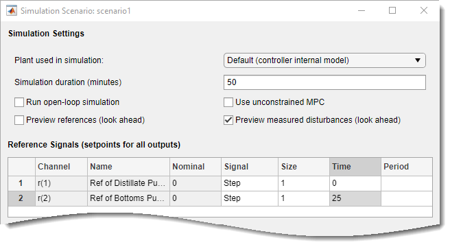
Click OK.
The app runs the simulation with the new scenario settings and updates the input and output response plots.
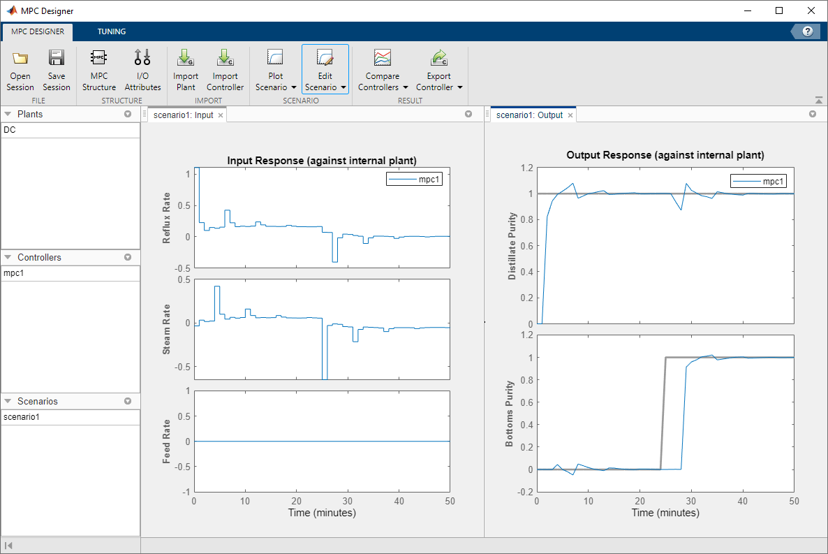
The Input Response plots show the optimal control moves generated
by the controller. The controller reacts immediately in response to the setpoint changes,
changing both manipulated variables. However, due to the plant delays, the effects of
these changes are not immediately reflected in the Output Response
plots. The Distillate Purity output responds after 1 minute, which
corresponds to the minimum delay from g11 and g12.
Similarly, the Bottoms Purity output responds 3 minutes after the
step change, which corresponds to the minimum delay from g21 and
g22. After the initial delays, both signals reach their setpoints and
settle quickly. Changing either output setpoint disturbs the response of the other output.
However, the magnitudes of these interactions are less than 10% of the step size.
Additionally, there are periodic pulses in the manipulated variable control actions as the controller attempts to counteract the delayed effects of each input on the two outputs.
Improve Performance Using Manipulated Variable Blocking
Use manipulated variable blocking to divide the prediction horizon into blocks, during which manipulated variable moves are constant. This technique produces smoother manipulated variable adjustments with less oscillation and smaller move sizes.
To use manipulated variable blocking, on the Tuning tab, specify
the Control horizon as a vector of block sizes, [5 5 5 5
10].
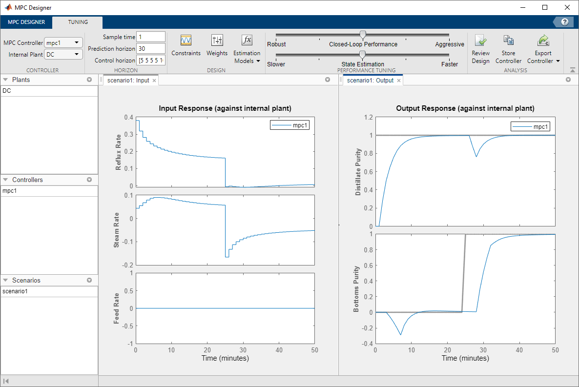
The initial manipulated variable moves are much smaller and the moves are less oscillatory. The tradeoff is a slower output response, with larger interactions between the outputs.
Improve Performance By Tuning Controller Weights
Alternatively, you can produce smooth manipulated variable moves by adjusting the tuning weights of the controller.
Set the Control horizon back to the previous value of
5.
In the Performance Tuning section, drag the Closed-Loop Performance slider to the left toward the Robust setting.
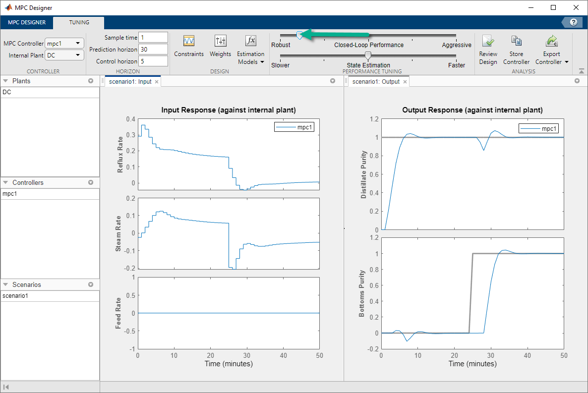
As you move the slider to the left, the manipulated variable moves become smoother and the output response becomes slower.
References
[1] Wood, R. K., and M. W. Berry, Chem. Eng. Sci., Vol. 28, pp. 1707, 1973.