Estimate Forest Fire Canopy Damage from Aerial Lidar Point Clouds

R2026b

Since R2026b

This example shows how to assess forest canopy damage caused by a wildfire using distance between pre-fire and post-fire aerial lidar point clouds.

Wildfires cause significant damage to forest canopies, and quantifying that damage is essential for post-fire recovery planning. Lidar point clouds captured before and after a fire provide detailed 3-D structural information about the canopy. By computing the nearest-neighbor distance between two temporally separated point clouds, you can identify areas of canopy loss and classify damage severity.

In this example, you:

• Download the USGS aerial point cloud data.

• Load and crop the point clouds to a region of interest.

• Downsample the point clouds to a uniform grid spacing.

• Compute distances between point clouds.

• Classify and visualize damage severity.

Download Point Cloud Data

In this example, you use lidar data from the U.S. Geological Survey (USGS) 3D Elevation Program (3DEP) publicly available through the USGS Lidar Explorer. This platform provides recorded lidar data in LAZ format for locations across the United States.

To see a real‑world change over time, download lidar data acquired before and after a wildfire event near Altadena and Pasadena, California. The pre‑fire data [1] was acquired in 2023, and the post‑fire data [2] was acquired in 2025 after the Eaton Fire. The websave function downloads each file if it does not already exist in your temporary folder. The tempdir command returns the location of this folder.

preFireLAZURL = "https://rockyweb.usgs.gov/vdelivery/Datasets/Staged/" + ...
    "Elevation/LPC/Projects/CA_LosAngeles_B23/CA_LosAngeles_1_B23/" + ...
    "LAZ/USGS_LPC_CA_LosAngeles_B23_11SMT040100378800.laz";

postFireLAZURL = "https://rockyweb.usgs.gov/vdelivery/Datasets/Staged/" + ...
    "Elevation/LPC/Projects/CA_2025LosAngelesPostWildfire_C25/CA_LAPostWildfire_Eaton_C25/" + ...
    "LAZ/USGS_LPC_CA_2025LosAngelesPostWildfire_C25_11SMT004012037875.laz";

lasDir = fullfile(tempdir,"fireEventLidarData");
if ~exist(lasDir,"dir")
    mkdir(lasDir)
end

preFireFile = fullfile(lasDir,"preFireData.laz");
if ~exist(preFireFile,"file")
    fprintf("Downloading preFireData.laz...\n")
    websave(preFireFile,preFireLAZURL,weboptions(Timeout=180));
end

Downloading preFireData.laz...

postFireFile = fullfile(lasDir,"postFireData.laz");
if ~exist(postFireFile,"file")
    fprintf("Downloading postFireData.laz...\n")
    websave(postFireFile,postFireLAZURL,weboptions(Timeout=180));
end

Downloading postFireData.laz...

Load and Crop Point Clouds

Create lasFileReader objects for the pre-fire and post-fire point cloud data, and use the readPointCloud object function to load the data from each file into the workspace. To crop the data to a 250-by-250 meter area within the damage perimeter, specify a region of interest (ROI) as a six-element vector of the form [xmin xmax ymin ymax zmin zmax].

roi = [401250 401500 3788000 3788250 -inf inf];

preFireReader = lasFileReader(preFireFile);
prePtCloud = readPointCloud(preFireReader,ROI=roi);
fprintf("Pre-fire points:  %d\n",prePtCloud.Count)

Pre-fire points:  1923153

postFireReader = lasFileReader(postFireFile);
postPtCloud = readPointCloud(postFireReader,ROI=roi);
fprintf("Post-fire points: %d\n",postPtCloud.Count)

Post-fire points: 3275645

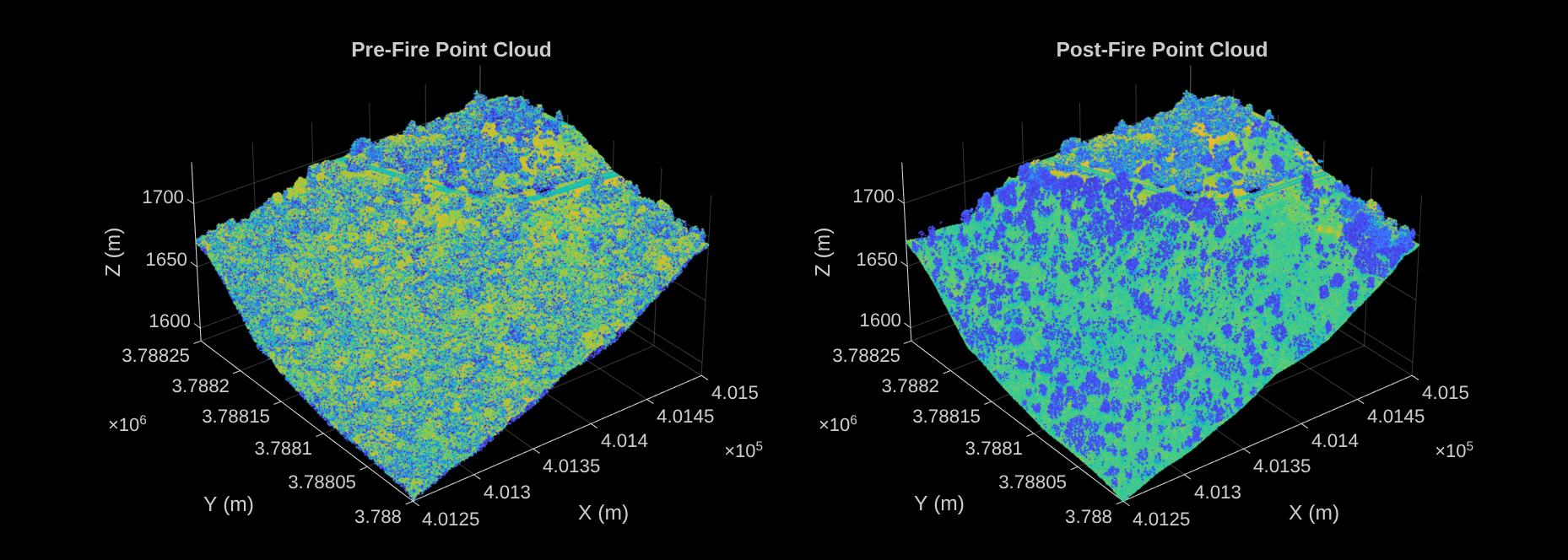
To visually compare the canopy structure before and after the fire, display the loaded point clouds next to each other. Use the pcshow function with intensity as the color source.

hFigPtDisplay = figure(Position=[100 100 1400 500]);
tPtDisplay = tiledlayout(hFigPtDisplay,1,2);                                                           

axPtDisplay1 = nexttile(tPtDisplay);
pcshow(prePtCloud,ColorSource="Intensity",Parent=axPtDisplay1)
title(axPtDisplay1,"Pre-Fire Point Cloud")
xlabel(axPtDisplay1,"X (m)")
ylabel(axPtDisplay1,"Y (m)")
zlabel(axPtDisplay1,"Z (m)")

axPtDisplay2 = nexttile(tPtDisplay);
pcshow(postPtCloud,ColorSource="Intensity",Parent=axPtDisplay2)
title(axPtDisplay2,"Post-Fire Point Cloud")
xlabel(axPtDisplay2,"X (m)")
ylabel(axPtDisplay2,"Y (m)")
zlabel(axPtDisplay2,"Z (m)")

Downsample Point Clouds

To improve the accuracy of point cloud distance computation, downsample both point clouds to a uniform grid spacing using the pcdownsample function. Downsampling reduces computational cost and ensures consistent point density between the two point clouds.

gridSize = 0.5; % meters
prePtCloud = pcdownsample(prePtCloud,gridAverage=gridSize);
postPtCloud = pcdownsample(postPtCloud,gridAverage=gridSize);

fprintf("After downsampling — Pre-fire points: %d, Post-fire points: %d\n", ...
    prePtCloud.Count,postPtCloud.Count)

After downsampling - Pre-fire points: 850747, Post-fire points: 589368

Compute Distance Between Point Clouds

To identify changes between the pre‑fire and post‑fire point clouds, compute the distance between them using the pcdistance function. For each point in the pre‑fire point cloud, the function finds the nearest neighbor in the post‑fire point cloud and returns the 3‑D Euclidean distance. Larger distances indicate areas where the canopy has been destroyed, while near‑zero distances indicate unchanged regions.

dists = pcdistance(prePtCloud,postPtCloud);

Classify and Visualize Damage Severity

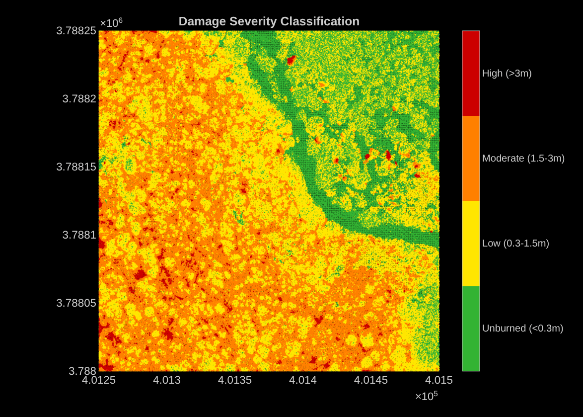
Classify each point into a damage severity category based on the distance between the two point clouds. The example uses these distance thresholds, but you can replace or adjust them based on your application.

• Unburned (< 0.3 m) — Canopy intact with negligible change.

• Low (0.3–1.5 m) — Minor canopy thinning or leaf loss.

• Moderate (1.5–3 m) — Significant canopy damage with partial loss.

• High (> 3 m) — Complete canopy destruction.

severityEdges  = [0 0.3 1.5 3 Inf];
severityLabels = ["Unburned (<0.3m)","Low (0.3-1.5m)", ...
    "Moderate (1.5-3m)","High (>3m)"];

nPtsPerClass = histcounts(dists,severityEdges);
nTotalPts = numel(dists);

Visualize the classified damage severity as a heatmap overlaid on the pre-fire point cloud using the pcheatmap function. The color scheme uses green for unburned areas, yellow for low severity, orange for moderate severity, and red for high severity.

severityColors = [0.2 0.7 0.2;    % Green  - Unburned
                  1.0 0.9 0.0;    % Yellow - Low
                  1.0 0.5 0.0;    % Orange - Moderate
                  0.8 0.0 0.0];   % Red    - High

classLabels = discretize(dists,severityEdges);

hFigSeverityMap = figure(Position=[100 100 700 500]);
axSeverityMap = axes(hFigSeverityMap);
pcheatmap(prePtCloud,classLabels,Colormap=severityColors, ...
    ViewPlane="XY",Projection="orthographic",Parent=axSeverityMap)
title(axSeverityMap,"Damage Severity Classification")
colorbarHandlecb = findobj(axSeverityMap.Parent,Type="ColorBar");
colorbarHandlecb.Ticks = colorbarHandlecb.Ticks(1:end-1) + diff(colorbarHandlecb.Ticks)/2;
colorbarHandlecb.TickLabels = severityLabels;
colorbarHandlecb.TickLength = 0;

Compute Summary Statistics

To characterize overall canopy change, compute summary statistics for the distance values. The mean and median distances indicate the typical level of change, while higher percentiles capture larger deviations associated with canopy loss.

stats.min    = min(dists);
stats.max    = max(dists);
stats.mean   = mean(dists);
stats.median = median(dists);
stats.std    = std(dists);
stats.rmse   = sqrt(mean(dists.^2));
stats.p95    = prctile(dists, 95);
stats.p99    = prctile(dists, 99);

fprintf("\n==== Distance Statistics ====\n" + ...
    "Min:    %.3f m | Max:    %.3f m\n" + ...
    "Mean:   %.3f m | Median: %.3f m\n" + ...
    "Std:    %.3f m | RMSE:   %.3f m\n" + ...
    "P95:    %.3f m | P99:    %.3f m\n", ...                                                                                                    
    stats.min,stats.max, ...
    stats.mean,stats.median, ...
    stats.std,stats.rmse, ...                                                                                                                    
    stats.p95,stats.p99);

==== Distance Statistics ====
Min:    0.004 m | Max:    6.911 m
Mean:   0.956 m | Median: 0.773 m
Std:    0.754 m | RMSE:   1.218 m
P95:    2.356 m | P99:    2.960 m

Estimate Affected Area and Volume Loss

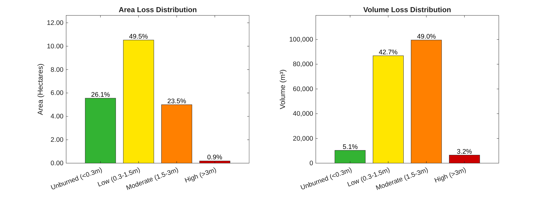
Estimate the area affected by each severity class and the volume of canopy material lost. Each downsampled point represents a grid cell of gridSize‑by‑gridSize meters. Estimate volume loss by summing the distance values for all points within each severity class and multiplying by the cell area.

areaPerPoint = gridSize^2;

totalAreaLoss = nTotalPts*areaPerPoint/10000;

totalVolLoss = sum(dists)*areaPerPoint;

areaPerClass = zeros(numel(severityLabels),1);
volPerClass = zeros(numel(severityLabels),1);
for i = 1:numel(severityLabels)
    areaPerClass(i) = nPtsPerClass(i)*areaPerPoint/10000;
    volPerClass(i) = sum(dists(classLabels==i))*areaPerPoint;
end

areaPercentage = 100*areaPerClass/totalAreaLoss;
volPercentage = 100*volPerClass/totalVolLoss;

hFigAreaAndVolLoss = figure(Position=[100 100 1400 500]);
tAreaAndVolLoss = tiledlayout(hFigAreaAndVolLoss,1,2);                                                                                                

axAreaLoss = nexttile(tAreaAndVolLoss);
bSeverityChart = bar(severityLabels,areaPerClass,FaceColor="flat", ...
    CData=severityColors,Parent=axAreaLoss);
bSeverityChart.Labels = compose("%.1f%%",areaPercentage);
ylabel(axAreaLoss,"Area (Hectares)")
ylim(axAreaLoss,[0 max(areaPerClass)*1.2])
ytickformat(axAreaLoss,"%,.2f")
xtickangle(axAreaLoss,20)
axAreaLoss.YAxis.Exponent = 0;
title(axAreaLoss,"Area Loss Distribution")

axVolumeLoss = nexttile(tAreaAndVolLoss);
bSeverityChart = bar(severityLabels,volPerClass,FaceColor="flat", ...
    CData=severityColors,Parent=axVolumeLoss);
bSeverityChart.Labels = compose("%.1f%%",volPercentage);
ylabel(axVolumeLoss,"Volume (m³)")
ylim(axVolumeLoss,[0 max(volPerClass)*1.2])
ytickformat(axVolumeLoss,"%,.0f")
xtickangle(axVolumeLoss,20)
axVolumeLoss.YAxis.Exponent = 0;
title(axVolumeLoss,"Volume Loss Distribution")

Visualize Pre-Fire and Post-Fire Cross-Sections

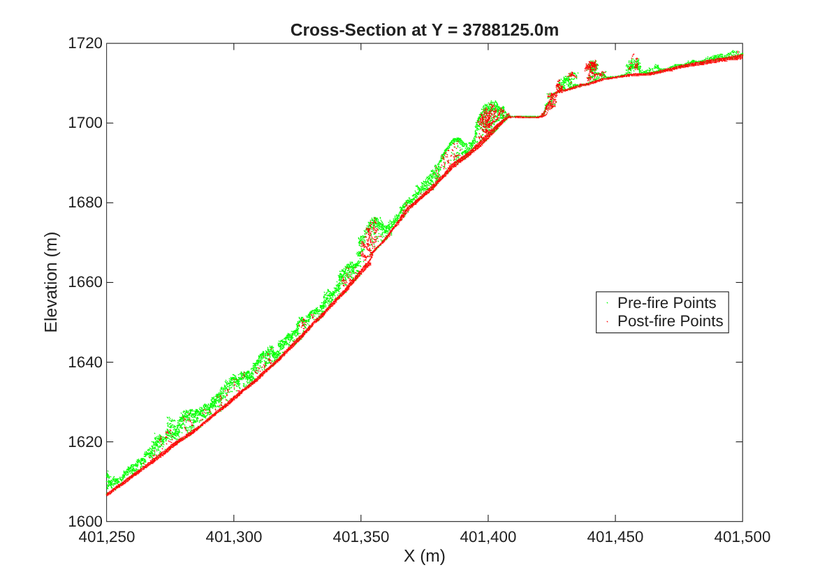
Extract a narrow cross-section slice through the center of the study area to compare the pre-fire and post-fire elevation profiles. This cross-section view highlights areas where the canopy has been damaged by fire, which appear as gaps between the green (pre-fire) and red (post-fire) points.

yMid = mean(prePtCloud.YLimits);

sliceWidth = 3.0;

preSliceROI = [prePtCloud.XLimits yMid-sliceWidth/2 yMid+sliceWidth/2 prePtCloud.ZLimits];
preSliceIds = findPointsInROI(prePtCloud,preSliceROI);
preSlice = select(prePtCloud,preSliceIds);

postSliceROI = [postPtCloud.XLimits yMid-sliceWidth/2 yMid+sliceWidth/2 postPtCloud.ZLimits];
postSliceIds = findPointsInROI(postPtCloud,postSliceROI);
postSlice = select(postPtCloud,postSliceIds);

hFigCrossSection = figure(Position=[100 100 700 500]);
axCrossSection = axes(hFigCrossSection);
plot(preSlice.Location(:,1),preSlice.Location(:,3),"g.", ...
    MarkerSize=2,DisplayName="Pre-fire Points",Parent=axCrossSection)
hold(axCrossSection,"on")

plot(postSlice.Location(:,1),postSlice.Location(:,3),"r.", ...
    MarkerSize=2,DisplayName="Post-fire Points",Parent=axCrossSection)
hold(axCrossSection,"off")

title(axCrossSection,sprintf("Cross-Section at Y = %.1fm",yMid))

axCrossSection.XAxis.Exponent = 0;
xtickformat(axCrossSection,"%,.0f")
xlabel(axCrossSection,"X (m)")
ylabel(axCrossSection,"Elevation (m)")
legend(axCrossSection,Location="best",FontSize=10)

[1] USGS Lidar Point Cloud CA_LosAngeles_B23 11SMT040100378800 courtesy of the U.S. Geological Survey

[2] USGS Lidar Point Cloud CA_2025LosAngelesPostWildfire_C25 11SMT004012037875 courtesy of the U.S. Geological Survey