Visualize LAS Classification Labels

R2026b

This example shows how to read classification attributes from a LAS file and color the point cloud by class in pcviewer. Point cloud data from collection methods like aerial surveys often includes per-point classification labels (ground, vegetation, buildings) following the ASPRS standard.

Download Data

Download a lidar tile from the USGS 3DEP NC Phase 2 survey covering downtown Wilson, North Carolina [1]. This tile contains approximately 8.5 million classified points.

tileURL = "https://rockyweb.usgs.gov/vdelivery/Datasets/Staged/" + ...
    "Elevation/LPC/Projects/NC_Phase2_2014/NC_WilsonCo_2014/LAZ/" + ...
    "USGS_LPC_NC_Phase2_2014_LA_37_20372101_.laz";
dataDir = fullfile(tempdir,"pcviewerClassificationData");
if ~exist(dataDir,"dir")
    mkdir(dataDir)
end
localFile = fullfile(dataDir,"wilsonDowntown.laz");
if ~exist(localFile,"file")
    websave(localFile, tileURL);
end

Read Point Cloud with Classification

Read the file using lasFileReader and readPointCloud. Use the Attributes argument to read the classification labels alongside the XYZ coordinates.

reader = lasFileReader(localFile);
[ptCloud, attr] = readPointCloud(reader, Attributes="Classification");
classLabels = attr.Classification;

Inspect Classification Labels

The ClassificationInfo property lists all classes present in the file along with their ASPRS standard names and point counts.

reader.ClassificationInfo

ans = 12×3 table
    Classification Value           Class Name            Number of Points by Class
    ____________________    _________________________    _________________________

              1             "Unclassified"                         123442         
              2             "Ground"                              3733928         
              3             "Low Vegetation"                        71601         
              4             "Medium Vegetation"                    211644         
              5             "High Vegetation"                      764755         
              6             "Building"                             728706         
              7             "Low Point(noise)"                       2743         
             11             "Road Surface"                            117         
             13             "Wire - Guard(Shield)"                 587630         
             14             "Wire - Conductor(Phase)"               10404         
             17             " Bridge Deck"                        1332922         
             18             "High Noise"                           916969         

	Get insights using Copilot

Visualize Ground, Vegetation, and Building classes to confirm they are classified correctly.

classes1 = [2 3 4 5 6];
names1 = ["Ground", "Low Vegetation", "Medium Vegetation", "High Vegetation", "Building"];
cmap = turbo(numel(classes1));
figure; hold on;
for i = 1:numel(classes1)
    pcshow(select(ptCloud, classLabels == classes1(i)).Location, repmat(cmap(i,:), nnz(classLabels == classes1(i)), 1));
end
legend(names1);

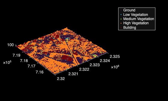
Ground, vegetation, and buildings are classified correctly. Now inspect the remaining classes.

classes2 = [11 13 14 17];
names2 = ["Road Surface", "Wire Guard", "Wire Conductor", "Bridge Deck"];
cmap = turbo(numel(classes2));
figure; hold on;
for i = 1:numel(classes2)
    pcshow(select(ptCloud, classLabels == classes2(i)).Location, repmat(cmap(i,:), nnz(classLabels == classes2(i)), 1));
end
legend(names2);

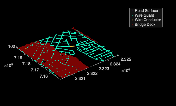
As visualized, Wire Guard (13) points are roads and Wire Conductor (14) points form a bridge deck. Road Surface (11) has too few points and Bridge Deck (17) overlaps with ground, and it is unclear what these points are. Remove noise, unclassified, and these two ambiguous classes, then relabel Wire Guard as "Road Surface" and Wire Conductor as "Bridge Deck" below.

Filter and Reclassify

unclassified = 1;
lowPoint = 7;
roadSurface = 11;
bridgeDeck = 17;
highNoise = 18;
removeClasses = [unclassified, lowPoint, roadSurface, bridgeDeck, highNoise];
keepIdx = ~ismember(classLabels, removeClasses);
ptCloud = select(ptCloud, keepIdx);
classLabels = classLabels(keepIdx);

Define Classification Colors

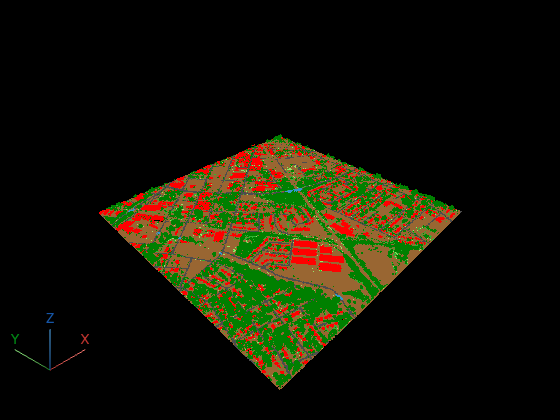
Map each remaining class ID to a distinct color. Relabel class 13 as "Road Surface" and class 14 as "Bridge Deck" based on the inspection above.

classIDs = [2, 3, 4, 5, 6, 13, 14];
classColorMap = [ ...
    0.6 0.4 0.2; ...  % Ground - brown
    0.6 0.9 0.4; ...  % Low Vegetation - light green
    0.2 0.7 0.2; ...  % Medium Vegetation - green
    0.0 0.5 0.0; ...  % High Vegetation - dark green
    1.0 0.0 0.0; ...  % Building - red
    0.3 0.3 0.3; ...  % Road Surface - dark gray
    0.2 0.6 0.8];     % Bridge Deck - blue

Build Per-Point Color Array and Visualize

Use ismember to map each classification label to a row in the color table, then index directly into the RGB matrix.

[~, idx] = ismember(classLabels, classIDs);
colors = classColorMap(idx, :);
pcviewer(ptCloud, colors);

References

[1] USGS Lidar Point Cloud NC_Phase2_2014 courtesy of the U.S. Geological Survey.