Introduction to Scanning and Processing Losses in Pulse Radar

In an idealized radar system with no losses and a nonfluctuating target, the detectability factor is a function of only three parameters — the desired probability of detection $$P_d$$, the required probability of false alarm $$P_{fa}$$, and the number of received pulses $$N$$. Practical systems, however, employ suboptimal processing resulting in a series of losses that must be added to the detectability factor. These losses increase the required signal energy needed to satisfy the stated detection requirements. Thus, the effective detectability factor becomes dependent on the components of the signal processing chain, the type of the pulse integration, the target fluctuation model, and several other factors. This example shows how various parameters influence the losses that must be included in the radar detectability factor when evaluating the radar equation. It discusses losses caused by the pulse eclipsing effect, off-broadside scanning with an electronic beam, and moving target indication (MTI) processing. It also addresses constant false alarm rate (CFAR) loss and filter matching loss.

The Modeling Radar Detectability Factors example discusses in detail the computation of the detectability factor for a radar system given a set of performance requirements. It shows how to use the detectability factor in the radar equation to evaluate the maximum detection range. It also shows how to compute the effective probability of detection at a given range.

Statistical Losses

The effective probability of detection, $$p$$, is a function of the available SNR at the receiver, $$\underset{}{\overset{‾}{\chi }}$$

$$p=p(\underset{}{\overset{‾}{\chi }})$$.

For a specific target position, the available SNR, $$\underset{}{\overset{‾}{{\chi }_0}}$$, can be computed from the radar equation, which typically assumes that the observed target is in the middle of a range-Doppler cell and lies directly along the antenna axis. However, since the target's position varies in the four-dimensional radar space, the probability of detection will also vary

$$p=p(\underset{}{\overset{‾}{{\chi }_0}}H(x))$$

where $$H(x)$$ is a scaling factor indicating the change in the available SNR when the target is located at a position $$x$$ in the range-Doppler-angle space. Thus, it makes sense to introduce the average probability of detection for a region bounded by the target positions $$x_1$$ and $$x_2$$

$$\underset{}{\overset{‾}{P}}=\frac{1}{x_2-x_1}{\int }_{x_1}^{x2}p(\underset{}{\overset{‾}{{\chi }_0}}H(x))dx$$

Here the probability that a target echo arrives from the position $$x$$ is assumed to be uniformly distributed between the boundaries $$x_1$$ and $$x_2$$. Thus, the SNR $$\underset{}{\overset{‾}{{\chi }_s}}$$ needed to achieve the required $$P_d$$ on average can be found by solving the following equation

$$P_d-\frac{1}{x_2-x_1}{\int }_{x_1}^{x_2}p(\underset{}{\overset{‾}{\chi }}H(x))dx=0$$

The increase in the SNR, $$\underset{}{\overset{‾}{{\chi }_s}}$$, compared to the idealized case when there are no probability of detection variations with $$x$$, is called a statistical loss [1]

$$L_s=\frac{\underset{}{\overset{‾}{{\chi }_s}}}{\underset{}{\overset{‾}{{\chi }_0}}}$$

This example considers three statistical losses:

• Eclipsing loss — Accounts for $$P_d$$ variations with range due to the pulse eclipsing effect.

• Array scan sector loss — Accounts for $$P_d$$ variations with a scan angle in electronically scanned arrays due the reduced projected array area in the beam direction and a reduction of the effective aperture area of the individual array elements at off-broadside angles.

• MTI velocity response loss — Accounts for $$P_d$$ variations due to a target lying close or in a null of the MTI filter.

Eclipsing Loss

Typically, pulse radar systems turn off their receivers during the pulse transmission. Thus, the target echoes arriving from the ranges within one pulse length from the radar or within one pulse length around the unambiguous range will be eclipsed by the transmitted pulse resulting in only a fraction of the pulse being received and processed. For different values of the duty cycle, the fraction of the received signal energy due to eclipsing is shown here as a function of the target range assuming the pulse repetition frequency (PRF) is 1kHz.

% Duty cycle
Du = [0.02 0.05 0.1 0.2];
 
% Pulse repetition frequency
PRF = 1e3;

% Compute eclipsing factor at 1 km intervals between zero and the
% unambiguous range
R = 0:1000:time2range(1/PRF);
Fecl = zeros(numel(R),numel(Du));
for i = 1:numel(Du)
    Fecl(:,i) = eclipsingfactor(R,Du(i),PRF);
end

% Plot the eclipsing factor in linear units
figure
plot(R*1e-3,db2pow(Fecl),'LineWidth',2)

xlabel('Range (km)')
ylabel('Received Energy Fraction')
title({'Eclipsing Effect',sprintf("PRF=%d Hz",PRF)})

legend(helperLegendLabels('Duty cycle = %.2f',Du),'location','south')
grid
ylim([0 1.2])

The variations in the received signal energy due to the eclipsing effect causes variations in the probability of detection. Specifically, $$P_d$$ decreases rapidly as a larger and larger fraction of the pulse is eclipsed when the target range approaches zero or the unambiguous range. The statistical eclipsing loss is computed as an increase in the signal energy required to compensate for these variations and make the probability of detection, averaged over the target ranges, equal to the desired probability of detection. Compute the statistical eclipsing loss as a function of $$P_d$$ for $$P_{fa}=10^{-6}$$ and different values of the duty cycle.

% Detection probability
Pd = linspace(0.1,0.99,100);

% Probability of false alarm
Pfa = 1e-6;

% Eclipsing loss
Lecl = zeros(numel(Pd),numel(Du));

for i = 1:numel(Du)
    % Assume a single pulse is received from a Swerling 1 target
    Lecl(:,i) = eclipsingloss(Pd,Pfa,1,Du(i),'Swerling1');
end

figure
plot(Pd,Lecl,'LineWidth',2)

xlabel('Detection Probability')
ylabel('Loss (dB)')
title({'Eclipsing Loss',sprintf('Swerling 1 Case, P_{fa}=%.0e',Pfa)})

legend(helperLegendLabels('Duty cycle = %.2f',Du),'location','northwest')
grid on

The statistical eclipsing loss increases with the duty cycle and can become very large for high values of $$P_d$$. This loss should be included in the radar equation when analyzing high-PRF radar systems in which a target can pass rapidly through the eclipsing regions. In such systems, the PRF diversity is typically used to mitigate the eclipsing effects by shifting the eclipsing regions in range.

Scan Sector Loss

In radar systems with electronically scanned phased array antennas, the gain of the antenna array scanned off broadside is reduced due to the reduction of the projected array area in the beam direction and the reduction of the effective aperture area of the individual array elements at off-broadside angles. Assuming both the transmitter and the receiver are using the same antenna array, at an off-broadside angle $$\theta$$ the received energy is reduced by approximately a factor of $${\cos }^3\theta$$.

theta = linspace(-90,90,500);

figure
plot(theta,cosd(theta).^3,'LineWidth',2)

xlabel('Scan Angle (deg)')
ylabel('cos^3(\theta)')
title('Reduction in Antenna Gain for a Phased Array Scanning off Broadside')
grid on

This figure shows that the received energy is reduced by half when the beam is pointed to about 37 degrees off broadsided.

The statistical scan sector loss defined for a scan sector $$[{\theta }_1,{\theta }_2]$$ is an increase in the signal energy required to obtain a specific value of the average $$P_d$$ over this scan sector compared to the signal energy required to obtain the same $$P_d$$ when the target lies along the antenna axis.

Consider scan sectors of different sizes and compute the statistical scan sector loss as a function of $$P_d$$ for $$P_{fa}=10^{-6}$$. The value of $$\theta$$ shown in the legend is the maximum scan angle specified about the broadside direction, that is the array scans from $$-\theta$$ to $$+\theta$$.

% Maximum scan angle about the broadside direction (deg)
Theta = [15 30 45 60];

% Array scan sector loss
Lscan = zeros(numel(Pd),numel(Theta));

for i = 1:numel(Theta)
    % Assume a single pulse is received from a Swerling 1 target
    Lscan(:,i) = arrayscanloss(Pd,Pfa,1,Theta(i),'Swerling1','CosinePower',3);
end

figure
plot(Pd,Lscan,'LineWidth',2)

xlabel('Detection Probability')
ylabel('Loss (dB)')
title({'Array Scan Sector Loss',sprintf('Swerling 1 Case, P_{fa}=%.0e',Pfa)})

legend(helperLegendLabels('\\theta = %.0f deg',Theta),'location','northwest')
grid on

For small scan sectors the statistical scan sector loss is relatively small and does not significantly vary with the probability of detection. As the size of the scan sector increases, the reduction in antenna gain becomes larger resulting in more rapid increase in the scan sector loss for larger values of the detection probability.

MTI Velocity Response Loss

In moving target indicator (MTI) radar systems, the MTI filter is used to reject clutter components at or near zero Doppler frequency or near the center frequency of the clutter spectrum while passing the target signal spectrum as much as possible. Because the MTI filter is not ideal, it can significantly suppress or even cancel the targets that are close to the null of its frequency response. To illustrate this, the frequency responses of the two, three, and four-pulse MTI cancellers are shown here.

m = [2 3 4];
fdnorm = linspace(-0.5,0.5,100);

% Frequency response of an m-pulse MTI canceller
Hmti = (2*sin(pi*fdnorm)) .^ (m'-1);

figure
plot(fdnorm,abs(Hmti),'LineWidth',2)

xlabel('Normalized Doppler Frequency')
ylabel('Frequency Response')
title('2, 3, and 4-pulse Canceller Frequency Response')

legend(helperLegendLabels('m = %d',m),'location','north')
grid on

To guarantee that the detection probability averaged over the Doppler frequencies of interest equals the required $$P_d$$, the average received signal energy must be increased. This increase compared to the energy required in a system without the MTI (with an all-pass filter) is called a statistical MTI velocity response loss. Plot the MTI velocity response loss as a function of $$P_d$$ for $$P_{fa}=10^{-6}$$.

Lmti_velocity_responce = zeros(numel(Pd),numel(m));

for i = 1:numel(m)
    [~,Lmti_velocity_responce(:,i)] = mtiloss(Pd,Pfa,m(i)+1,m(i),'Swerling1');
end

figure
plot(Pd,Lmti_velocity_responce,'LineWidth',2)

xlabel('Detection Probability')
ylabel('Loss (dB)')
title({'MTI Velocity Response Loss',sprintf('Swerling 1 Case, P_{fa}=%.0e',Pfa)})

legend(helperLegendLabels('m = %d',m),'location','northwest')
grid on
ylim([-1 10])

This result shows that in the MTI system with a single PRF the statistical velocity response loss can become very large. The loss grows with the probability of detection. It also increases as the order of the MTI filter increases since the stop band of the filter becomes broader. In practical systems, staggered PRF is used to prevent large values of the MTI velocity response loss.

MTI Integration Loss

In addition to the MTI velocity response loss, the MTI system has another category of losses that must be taken into account. These losses could be viewed as a reduction in the effective number of pulses available for integration after the MTI. Depending on the type of the MTI processing these losses can include [1]:

• MTI noise correlation loss. This loss is a result of the partial correlation introduced by the MTI processing to the received pulses that pass through an $$m$$-pulse MTI canceller.

• MTI batch processing loss. The result of using a batch processing MTI instead of a sequential MTI. A batch MTI processes $$N$$ received pulses in batches of size $$m$$ resulting in only $$N/m$$ pulses available for integration at the output of the MTI.

• MTI blind phase loss. If only a single channel is available for the MTI processing, the number of available independent target samples is reduced by a factor of two. Additionally, the fluctuation loss also increases. This loss must be added to the noise correlation loss.

To compare different components of the MTI integration loss, consider two, three, and four-pulse MTI cancellers. The probability of detection is set to $$P_d=0.9$$ and the probability of false alarm to $$P_{fa}=10^{-6}$$.

% Number of pulses in MTI canceller
m = [2 3 4];

% Detection probability
Pd = 0.9;

% Probability of false alarm
Pfa = 1e-6;

The losses are computed for Swerling 1 case and are plotted as a function of the number of received pulses $$N$$. Consider a quadrature MTI with sequential processing, a quadrature MTI with batch processing, and a single-channel MTI with sequential processing.

% Number of received pulses
N = 1:100;

% MTI noise correlation loss
Lmti_noise_correlation = NaN(numel(m),numel(N));

% MTI blind phase loss
Lmti_blind_phase = NaN(numel(m),numel(N));

% MTI batch processing loss
Lmti_batch_processing = NaN(numel(m),numel(N));

% Compute losses
for i = 1:numel(m)
    for j = 1:numel(N)
        if N(j) > m(i)
            [Lnc,~,Lbp] = mtiloss(Pd,Pfa,N(j),m(i),'Swerling1','IsQuadrature',false);
            Lmti_noise_correlation(i,j) = Lnc;
            Lmti_blind_phase(i,j) = Lbp + Lnc;

            Lnc = mtiloss(Pd,Pfa,N(j),m(i),'Swerling1','Method','batch');
            Lmti_batch_processing(i,j) = Lnc;
        end
    end
end

% Plot results
figure
for i = 1:numel(m)
    subplot(3,1,i)
    semilogx(N,Lmti_noise_correlation(i,:),'LineWidth',2)
    hold on
    semilogx(N,Lmti_batch_processing(i,:),'LineWidth',2)
    semilogx(N,Lmti_blind_phase(i,:),'LineWidth',2)
    
    ylabel('Loss (dB)')
    title(sprintf('%d-pulse Canceller',m(i)))
    
    set(gca(),'xtick',xticks,'xticklabel',num2cell(xticks))
    legend({'Quadrature','Batch','Single-channel'},'location','northeast')
    grid on
    ylim([0 8])
end

xlabel('Number of Received Pulses')
set(gcf,'Position',[100 100 800 600])

From these results we can see that the quadrature MTI with sequential processing is the most efficient. The noise correlation loss decreases as more pulses become available for integration. For the batch processing MTI, the loss is close to the sequential case when the number of received pulses is small. It also decreases with $$N$$ but not as fast. Finally, the blind phase loss due to a single-channel MTI is the largest because in this case the number of available samples is further decreased by two in addition to the noise correlation loss.

CFAR Loss

CFAR is used to estimate the value of the detection threshold when the levels of the noise or clutter are variable. In practice, however, this estimate is subject to an error due to the finite number of reference cells, $$n_{cells}$$, and the rapid changes in the interference levels. To compensate for this error a higher received signal energy is needed. The increase in the signal energy required to achieve the desired detection performance using CFAR compared to a system with a perfectly known detection threshold is called a CFAR loss. For a one-dimensional case, a convenient approximation for CFAR loss in cell-averaging (CA) and greatest-of cell-averaging (GOCA) CFAR was developed in [3] and described in [1].

% Number of CFAR reference cells
numCells = 4:4:64;

% Probability of false alarm
Pfa = 1e-8;

% CFAR ratio
x = -log10(Pfa)./numCells;

% Compute CFAR loss
Lcfar_ca = cfarloss(Pfa,numCells);
Lcfar_goca = cfarloss(Pfa,numCells,'Method','GOCA');

% Plot
figure
hold on
plot(x,Lcfar_ca,'LineWidth',2)
plot(x,Lcfar_goca,'LineWidth',2)

xlabel('-log10(P_{fa})/n_{cells}')
ylabel('Loss (dB)')
title({'Universal Curve for CFAR Loss'})

legend({'Cell-averaging','Greatest-of cell-averaging'},'location','northwest')
grid on

For a given CFAR method, the approximated loss depends only on the ratio $$-lo{g}_{10}(P_{fa})/n_{cells}$$, called a CFAR ratio. This allows for finding a trade-off between the required probability of false alarm and the number of reference cells to achieve a desired level of CFAR loss. The approximation shows that CFAR loss increases with the CFAR ratio. The loss of about 2 dB or smaller can be achieved if the CFAR ratio is kept under 0.4 for both CA and GOCA CFAR methods. If $$n_{cells}$$ is kept constant, reducing $$P_{fa}$$ would result in an increased loss. Thus, to achieve a lower required probability of false alarm while keeping the loss small, the number of reference cells must be increased. These loss curves are referred to as universal curves for CFAR loss since they can be used both for nonfluctuating and Rayleigh targets and need only $$P_{fa}$$ and $$n_{cells}$$ to compute the loss. This makes it easy to use these results when analyzing a wide variety of radar systems [1].

Matching Loss

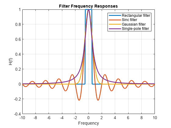
When the spectrum of the received signal is different from the spectrum of the matched filter, the system will incur a matching loss. This loss can be defined as a ratio of the received output SNR to the SNR available from a filter perfectly matched to the received signal. This example considers several filter types: rectangular, Sinc, Gaussian, and single-pole. For ease of comparison, the filter bandwidth is assumed to be equal to one. The shapes of these filters are shown in the following figure.

% Normalized bandwidth of the matched filter
B = 1;

% Max normalized pulse duration
taumax = 10;

% Sampling period
dt = 0.01;

% Number of frequency bins
nf = 2 ^ (nextpow2(taumax/dt) + 1);
m = -nf/2:nf/2 - 1;

% Normalized frequency
f = m / (nf*dt);
H = zeros(4,numel(f));

% Frequency response of a rectangular filter
H(1,abs(f) <= B/2) = 1;

% Frequency response of a sinc filter
H(2,:) = sinc(f/B);

% Frequency response of a Gaussian filter
H(3,:) = exp(-(pi/2) * (f/B).^2);

% Frequency response of a single-pole filter
H(4,:) = 1./(1 + (pi*f / (2*B)).^2);

figure
plot(f,H,'LineWidth',2)

xlabel('Frequency')
ylabel('H(f)')
title('Filter Frequency Responses')

labels = {'Rectangular filter','Sinc filter','Gaussian filter','Single-pole filter'};
legend(labels)
grid on;
xlim([-10 10])

The received signal in this example is an unmodulated ideal rectangular pulse. The filter matching loss for the four filter types is shown here as a function of the time-bandwidth product.

% Pulse duration normalized by (1/B)
tau = 0.1:0.1:taumax;

% Spectrum of an ideal pulse with no phase modulation
N = ceil(tau.'/dt);
S = sin(pi*N*m/nf) ./ sin(pi*m/nf);
S(:,nf/2 + 1) = N;

% Matching loss
L = matchingloss(S,H);

figure
semilogx(tau*B,L,'LineWidth',2)

xlabel('Time-Bandwidth Product')
ylabel('Loss (dB)')
title({'Matching Loss for an Unmodulated Rectangular Pulse'})

legend(labels,'location','North')
xticks = [0.1 0.2 0.5 1 2 5 10];
set(gca(),'xtick',xticks,'xticklabel',num2cell(xticks))
grid on

As expected, the filter with the Sinc spectrum has the lowest matching loss because it ideally matches the spectrum of the unmodulated rectangular pulse. The Gaussian filter that can represent a cascade of several filters, results in 0.5 dB matching loss when the time-bandwidth product is close to 0.8.

Conclusion

This example discusses several losses that must be included in the effective detectability factor when evaluating the radar range equation. It starts by considering a category of statistical losses. These losses are incurred by a radar system because of a dependance of the effective detection probability on the target position in the range-Doppler-angle space. Evaluation of statistical losses due to the eclipsing effect, the off-broadside electronic scanning, and a nonideal MTI filter is shown in this example. It is also shown that these losses increase rapidly with the probability of detection. The example further explores losses in an MTI system by considering different components of the MTI integration loss and its dependence on the order of the MTI pulse canceller. The example also illustrates a convenient way to assess the CFAR loss based on the universal curve for CFAR loss. Finally, it shows the computation of the filter matching loss.

References

1. Barton, David Knox. Radar Equations for Modern Radar. Artech House, 2013.

2. Richards, M. A. Fundamentals of Radar Signal Processing. Second edition, McGraw-Hill Education, 2014.

3. Gregers-Hansen, V., "Constant false alarm rate processing in search radars." In IEE Conf. Publ. no. 105," Radar-Present and Future", pp. 325-332. 1973.