Train LSPI Agent to Balance Discrete Cart-Pole System

This example shows how to train an online least-squares policy iteration (LSPI) agent to balance a discrete action space cart-pole system modeled in MATLAB®. For more information on LSPI agents, see LSPI Agent.

Fix Random Number Stream for Reproducibility

The example code might involve computation of random numbers at several stages. Fixing the random number stream at the beginning of some sections in the example code preserves the random number sequence in the section every time you run it, which increases the likelihood of reproducing the results. For more information, see Results Reproducibility.

Fix the random number stream with seed 0 and random number algorithm Mersenne Twister. For more information on controlling the seed used for random number generation, see rng.

previousRngState = rng(0,"twister");

The output previousRngState is a structure that contains information about the previous state of the stream. You will restore the state at the end of the example.

Discrete Action Space Cart-Pole MATLAB Environment

The reinforcement learning environment for this example is a pole attached to an unactuated joint on a cart that moves along a frictionless track. The training goal is to make the pole stand upright.

For this environment:

• The upward balanced pole position is 0 radians, and the downward hanging position is pi radians.

• The pole starts upright with an initial angle between –0.05 and 0.05 radians.

• The force action signal from the agent to the environment is either –10 or 10 N.

• The observations from the environment are the position and velocity of the cart, pole angle, and pole angle derivative.

• The episode terminates if the pole is more than 12 degrees from vertical or if the cart moves more than 2.4 m from the original position.

• A reward of +1 is provided for every time step that the pole remains upright. A penalty of –5 is applied when the pole falls.

For more information on this model, see Load Predefined Control System Environments.

Create Environment Object

Create a predefined cart-pole environment object.

env = rlPredefinedEnv("CartPole-Discrete")

env = 
  CartPoleDiscreteAction with properties:

                  Gravity: 9.8000
                 MassCart: 1
                 MassPole: 0.1000
                   Length: 0.5000
                 MaxForce: 10
                       Ts: 0.0200
    ThetaThresholdRadians: 0.2094
               XThreshold: 2.4000
      RewardForNotFalling: 1
        PenaltyForFalling: -5
                    State: [4×1 double]

The interface has a discrete action space where the agent can apply one of two possible force values to the cart, –10 or 10 N.

Get the observation and action specification information.

obsInfo = getObservationInfo(env)

obsInfo = 
  rlNumericSpec with properties:

     LowerLimit: -Inf
     UpperLimit: Inf
           Name: "CartPole States"
    Description: "x, dx, theta, dtheta"
      Dimension: [4 1]
       DataType: "double"

actInfo = getActionInfo(env)

actInfo = 
  rlFiniteSetSpec with properties:

       Elements: [-10 10]
           Name: "CartPole Action"
    Description: [0×0 string]
      Dimension: [1 1]
       DataType: "double"

Create LSPI Agent

Fix the random stream for reproducibility.

rng(0,"twister");

LSPI agents use Q-value functions with basis functions as critics. This Q-value function represents the expected cumulative long-term reward for taking the corresponding discrete action from the state indicated by the observation inputs. For more information on creating value functions, see Create Policies and Value Functions. This examples uses myCartpoleBasisFcn as a basis function. The file containing this function is provided in the example folder.

type myCartPoleBasisFcn.m

function feature = myCartPoleBasisFcn(obs,act)
    % A basis function for a cartpole problem.
    
    % Copyright 2024 The MathWorks Inc.

    act = act/10;
    feature = [
        obs
        act
        obs.^2
        act.^2
        obs(1,1,:).*obs(2,1,:)
        obs(1,1,:).*obs(3,1,:)
        obs(1,1,:).*obs(4,1,:)
        obs(2,1,:).*obs(3,1,:)
        obs(2,1,:).*obs(4,1,:)
        obs(3,1,:).*obs(4,1,:)
        obs(1,1,:).*obs(2,1,:).*act
        obs(1,1,:).*obs(3,1,:).*act
        obs(1,1,:).*obs(4,1,:).*act
        obs(2,1,:).*obs(3,1,:).*act
        obs(2,1,:).*obs(4,1,:).*act
        obs(3,1,:).*obs(4,1,:).*act
        obs.*act];
end

This choice approximates the Q-value function as a polynomial. The linear, quadratic, and cross-product monomials capture curvature and smooth nonlinear relationships between the cart-pole's state and action. Other choices are possible, such as radial basis functions, and might produce an even better approximation of the optimal Q-value function.

Construct a Q-value function using myCartpoleBasisFcn.

% Compute the number of features.
obs = zeros(4,1);
act = 10;
temp = myCartPoleBasisFcn(obs, act);
numFeatures = numel(temp);

% Initialize weights.
w0 = rand(numFeatures, 1);

% Create a critic object.
critic = rlQValueFunction({@myCartPoleBasisFcn,w0},obsInfo, actInfo);

Specify the agent options for training using rlLSPIAgentOptions and rlOptimizerOptions objects. For this training, set LearningFrequency to 10 to update the critic every 10 samples collected.

agentOpts = rlLSPIAgentOptions(LearningFrequency=10);

LSPI agents use the epsilon-greedy algorithm to explore the action space during training. Specify a decay rate of 2e-4 for the epsilon value to gradually decay during training. This decay rate promotes exploration toward the beginning when the agent does not have a good policy, and exploitation toward the end when the agent has learned the optimal policy.

agentOpts.EpsilonGreedyExploration.EpsilonDecay = 2e-4;
agentOpts.EpsilonGreedyExploration.EpsilonMin = 0.05;

Create the LSPI agent using the observation and action input specifications, initialization options and agent options.

rng(0,"twister");
agent = rlLSPIAgent(critic,agentOpts);

For more information, see rlLSPIAgent.

Check the action of the agent with a random observation input.

getAction(agent,{rand(obsInfo.Dimension)})

ans = 1×1 cell array
    {[10]}

Train Agent

Fix the random stream for reproducibility.

rng(0,"twister");

To train the agent, first specify the training options. For this example, use these options:

• Run the training for a maximum of 1000 episodes, with each episode lasting a maximum of 500 time steps.

• Display the training progress in the Reinforcement Learning Training Monitor window (set the Plots option) and disable the command line display (set the Verbose option to false).

• Evaluate the performance of the greedy policy every 50 training episodes, averaging the cumulative reward of 5 simulations.

• Stop the training when the evaluation score reaches 500. At this point, the agent can balance the cart-pole system in the upright position.

% Training options
trainOpts = rlTrainingOptions( ...
    MaxEpisodes=3000, ...
    MaxStepsPerEpisode=500, ...
    Verbose=false, ...
    Plots="training-progress", ...
    StopTrainingCriteria="EvaluationStatistic", ...
    StopTrainingValue=500);

% Agent evaluator
evl = rlEvaluator(EvaluationFrequency=50,NumEpisodes=5,RandomSeeds=1:5);

For more information, see rlTrainingOptions and rlEvaluator.

Train the agent using the train function. Training this agent is a computationally intensive process that takes several minutes to complete. To save time while running this example, load a pretrained agent by setting doTraining to false. To train the agent yourself, set doTraining to true.

doTraining = false;
if doTraining
    % Train the agent.
    trainingStats = train(agent,env,trainOpts,Evaluator=evl);
else
    % Load the pretrained agent for the example.
    load("MATLABCartpoleLSPI.mat","agent")
end

Simulate Agent

Fix the random stream for reproducibility.

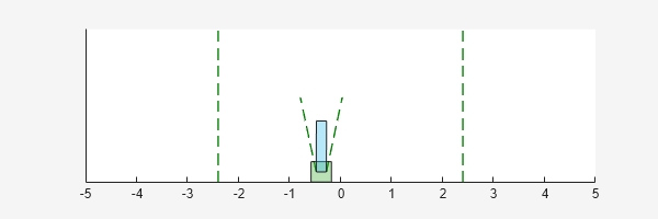
rng(0,"twister");

You can visualize the cart-pole system by using the plot function.

plot(env)

To validate the performance of the trained agent, simulate it within the cart-pole environment. For more information on agent simulation, see rlSimulationOptions and sim.

agent.UseExplorationPolicy = false;
simOptions = rlSimulationOptions(MaxSteps=500);
experience = sim(env,agent,simOptions);

totalReward = sum(experience.Reward)

totalReward = 
500

The agent can balance the cart-pole system.

Restore the random number stream using the information stored in previousRngState.

rng(previousRngState);