Simulate the Yeast Heterotrimeric G Protein Cycle
This example shows how to configure simulation settings, add an event to the model to trigger a time-based change, save, and plot the simulation results. This example uses the model described in Model of the Yeast Heterotrimeric G Protein Cycle to illustrate model simulation.
Load the gprotein.sbproj project, which includes the
variable m1, a SimBiology® model object.
sbioloadproject gproteinSet the simulation solver to ode15s and set a stop time of
500 by editing the SolverType and
StopTime properties of the configset
object associated with the m1 model.
csObj = getconfigset(m1);
csObj.SolverType = 'ode15s';
csObj.StopTime   = 500;
Specify to log simulation results of all species.
csObj.RuntimeOptions.StatesToLog = 'all';Suppose the amount of the ligand species L is 0 at the
start of the simulation, but it increases to a particular amount at time = 100.
Use sbioselect to select the
species named L and set its initial amount to 0. Use
addevent to set up the desired
event.
speciesObj = sbioselect(m1,'Type','species','Name','L');
speciesObj.InitialAmount = 0;
evt = addevent(m1,'time >= 100','L = 6.022E17');
Simulate the model.
[t,x,names] = sbiosimulate(m1);
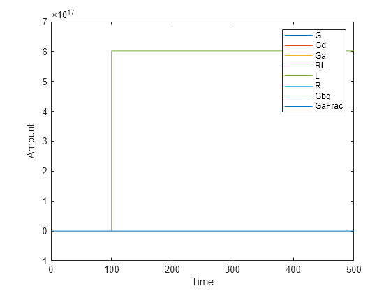
Simulate the simulation results. Notice that the species L amount increases when the event is triggered at simulation time 100. Changes in other species do not show up in the plot due to the wide range in species amounts.
plot(t,x);
legend(names)
xlabel('Time');
ylabel('Amount');
To see the changes of other species, plot without the species L (the 5th species) data.
figure
plot(t,x(:,[1:4 6:8]));
legend(names{[1:4 6:8]});
xlabel('Time');
ylabel('Amount');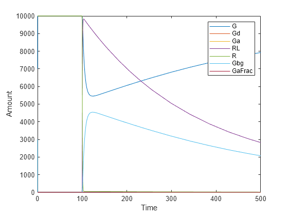
Alternative to storing simulation data in separate outputs, such as
t, x, and names as
above, you can store them all in a single SimData object. You can then
use selectbyname to extract arrays
containing the simulation data of your interest.
simdata     = sbiosimulate(m1);
sbioplot(simdata);
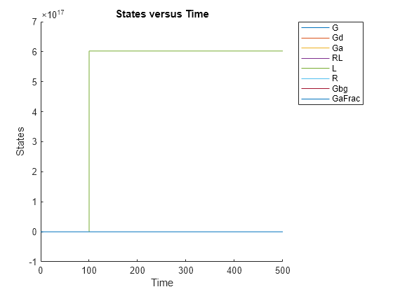
Expand Run 1 to see the names of species and parameter that are plotted.
simdata_noL = selectbyname(simdata, {'Ga','G','Gd','GaFrac','RL','R'});
sbioplot(simdata_noL);