Interpreting Angle in the Angle-Based Rotational Domain

Open Live Script

This example shows how to set up and interpret angles in angle-based rotational models. It provides background information to explain the underlying concepts. The angle-based rotational domain tracks angle, θ, and rotational velocity, ω, at every node. Use angle-based rotational blocks to model rotational systems where knowing multiple component angles is important.

This example describes how to:

Map views of the real physical system to the Simscape™ schematic.
Place blocks on the Simulink® canvas.
Define the positive rotational direction around an axis.
Specify angles in blocks.
Use a Rotational Motion Sensor (AB) block to wrap angle measurements.

The example uses three models to demonstrate the concepts:

The model in the image below shows the final result of the concepts covered in this example. The models you’ll see here are simple, but they demonstrate the workflow you can use to track systems with important angle-dependent behavior.

open_system('InterpretingAngleDiscsOnCompliantShaft');

Motion and Views in the Real System and Simscape Schematic

Concept 1: Motion

The angle-based rotational domain represents systems where components rotate around a fixed axis. The simulation computes the angle, θ, and angular velocity, ω, at every node in the network. This image shows two discs that can rotate around the fixed axis.

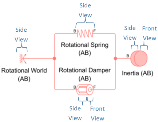
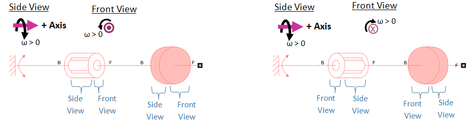
Concept 2: Physical View vs. Schematic View

A physical view shows what the system looks like in real life. A schematic view is how the Simscape network appears on the Simulink canvas.

A single schematic view can correspond to multiple physical views (front, back, side, or isometric).
The schematic view represents a side view of the axis. It is shown in an “exploded” layout so that components acting between the same axis locations appear in parallel.

This image shows four different physical views of the two discs on the axis and the corresponding Simscape schematic. Simscape models the two freely spinning discs using a Rotational World (AB) block, two Initial Relative Angle (AB) blocks, and two Inertia (AB) blocks.

Concept 3: Define the axis direction in your physical view and schematic view

The axis is a straight line in space with a defined positive direction. Rotational motion occurs around this line following the right-hand rule.

Choose the positive axis direction for your physical system and also for the Simscape schematic. These directions do not need to match—the physical view and schematic can use different orientations.

In this image:

The axis points to the right in both the isometric and side physical views.
The axis points into the page in the back physical view and out of the page in the front physical view.
In the Simscape schematic, the axis points to the right.

Placing Components Along an Axis in the Simscape Schematic

Concept 4: Arrange Components Along an Axis in the Simscape Schematic

In the Simscape schematic:

You place blocks along an axis to represent the physical system.
The order of the blocks along this axis reflects the sequence of components in the real-world layout. This is called axial ordering.
Blocks that appear closer to the tail of the axis have an earlier axial ordering, while blocks closer to the arrowhead have a later axial ordering.
Connections run along the axis, and rotational dynamics propagate through these connections.

The schematic shows connections along the axis, but Simscape only simulates rotational variables (angle θ and angular velocity ω).

Block ports connected to the same node are rigidly attached to each other.
They share an angle θ, and angular velocity ω, but they do not need to share the same axial location.
To model multiple components acting between two other components, connect them in parallel.

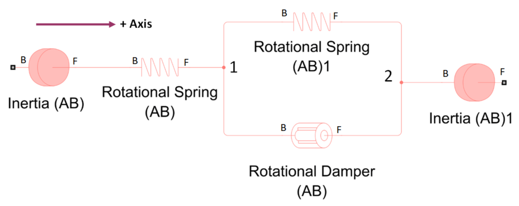
In this image:

The yellow disc appears later in the axial ordering (closer to the arrowhead), so it comes after the blue disc in the sequence from axis tail to arrowhead.
In the Simscape schematic, the Rotational Spring (AB) and Rotational Damper (AB) are connected in parallel and act between nodes 1 and 2.

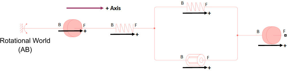
Concept 5: Align Components with the Positive Direction of the Axis in the Simscape Schematic

Two-port blocks have an internal positive direction from port B to port F.

For intuitive mapping of motion/torque behavior between the schematic and physical system, align this internal direction with the axis positive direction.

For more details on torque interpretation, see the Interpreting Torque in the Angle-Based Rotational Domain.

Block orientation on the canvas does not affect simulation results—only connectivity matters. However, consistent orientation makes it easier to relate simulation values to real-world behavior.

In this image:

The pink arrow shows the axis pointing to the right.
All two-port blocks are oriented with port B on the left and port F on the right, so their internal positive direction matches the axis direction.

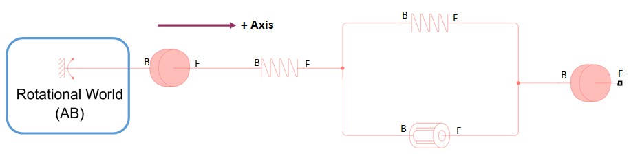
Concept 6: The Rotational World (AB) Block Sets the Stationary Reference Frame in the Simscape Schematic

The Rotational World (AB) block defines the absolute zero angle and angular velocity for the network.

At its node, both θ and ω equal zero.
All other node angles are measured relative to this block.

A rotational network can include multiple Rotational World (AB) blocks to represent different stationary points with zero angle.

To specify a stationary point with a nonzero angle, connect a Rotational Spacer (AB) block to a Rotational World (AB) block.

Defining Angles of Components

Concepts 7–9 are provided to help you visualize how the model represents motion in space. These concepts are for interpretation only—they do not change how Simscape simulates the system.

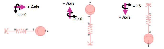
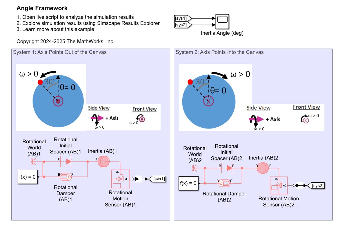
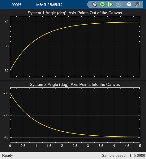
Concept 7: Visualize Rotation with the Right-Hand Rule

In both the physical view and the Simscape schematic, think about rotational motion as following the right-hand rule around the axis:

Point right thumb points in the positive axis direction.
Your curled fingers show the direction of positive rotation.

This image illustrates the right-hand rule for schematics for three different axes:

Axis pointing to the right
Axis pointing downward
Axis pointing upward

Each example shows how the positive rotational velocity (ω) relates to the axis direction.

Important notes:

It does not matter whether you choose the right-hand or left-hand rule—the key is to be consistent throughout your model.
Simscape does not apply either rule internally; it only records whether rotation and torque are positive or negative.
Use the rule as a visual aid to interpret simulation results, especially in complex systems.

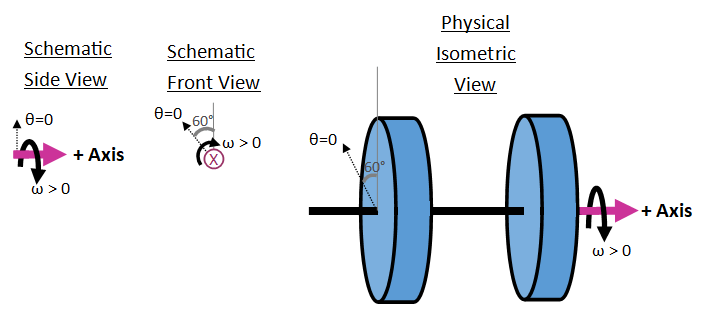
Concept 8: Define the θ = 0 Direction in the Physical View

In addition to defining the positive axis direction, you also define a stationary direction to represent an angle of 0 deg in your physical view.

This direction is a vector perpendicular to the axis and remains constant along the entire axis.
In this example, the $θ = 0$ direction points –60° from vertical.

The variable theta that Simscape logs for each node equals 0 when the node aligns with the $θ = 0$ direction.

This concept is for interpreting the physical view—it is not a setting you configure in the Simscape schematic.

Your choice of the $θ = 0$ direction affects how you set initial conditions in the schematic so they match your physical system.

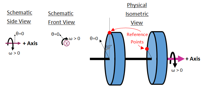
Concept 9: Choose Tracking Points on Axisymmetric Components in the Physical View

For axisymmetric components, such as Inertia (AB) and Rotational Damper (AB):

Choose a tracking point at a nonzero radial location on the component.
This point rotates with the component.
When the tracking point aligns with the $θ = 0$ line, the component's angle is 0, and the Simscape node variable theta equals 0.

In this image:

The left inertia (blue) has an angle of $θ = 60$ degrees.
The right inertia has an angle of $θ = 20$ degrees.

This tracking point concept is only for interpreting the physical view- it is not something you configure in Simscape.

For non-axisymmetric components (such as Rotational Hard Stop (AB)), the block ports already correspond to specific physical locations where the component connects to the system. Therefore, you do not need to define a tracking point.

Block-Specific Angle Behaviors

The theta variable at each block node tracks the simulated angle versus time. To initialize angles in a model, set the Relative angle variable in two-port blocks.

Concept 10: Two-Port Blocks with Varying Angles Between Ports

For some two-port blocks, the angle between the ports can change during the simulation.

This angle is tracked by the Relative angle variable: theta_rel = F.theta - B.theta.
You can set the initial value of Relative angle on the Initial Targets tab of the dialog box.

These blocks include:

Rotational Spring (AB)
Rotational Damper (AB)
Rotational Friction (AB)
Rotational Hard Stop (AB)
Rotational Inerter (AB).

Example: The Model of Discs on a Compliant Shaft uses the Rotational Spring (AB) and Rotational Damper (AB).

Concept 11: Two-Port Blocks with Ports at the Same Angle

Some two-port blocks always keep both ports at the same angle.

These blocks show two ports so the schematic can display a continuous axis line when the block is placed in the middle of the axis.
These blocks can display one port for visual neatness when the block is at the end of the axis.

These blocks include:

Inertia (AB)
Inertia With Friction (AB)
Wheel and Axle (AB-PB)
Cam and Follower (AB-PB)

Example models with Inertia (AB):

Concept 12: Use an Initial Relative Angle (AB) block to Set an Initial Condition

Use an Initial Relative Angle (AB) block to define an initial angle between two points. This block is only for setting initial conditions. It does not represent a physical component, apply torque, or affect the simulation after the first time step. It also does not include angle-wrapping effects.

When defining many initial angles, use the Initial Relative Angle (AB) block to specify angles between non-World components, rather than specifying multiple angles relative to the World (AB) block. Specifying angles between non-World components helps keep the model more flexible and adaptable.

Example models with Initial Relative Angle (AB):

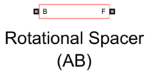
Concept 13: Rotational Spacer (AB) Block Maintains a Fixed Angle Offset Throughout Simulation

The Rotational Spacer (AB) block enforces a constant angular offset between two points throughout the simulation. The Rotational Spacer represents a real, rigid component of the system.

The spacer ports B and F have the same angular velocity: $ω_{F} = ω_{B}$ . Their angles differ by a constant offset equal to the Relative angle parameter: $θ_{r e l} = θ_{F} - θ_{B}$ .

There are two ways to use a spacer block:

In series: It apples a fixed angle offset between two points on a rigid body.
In parallel with multiple blocks: It enforces an angle constraint across the blocks. If the Rotational World (AB) block is connected to one of the spacer ports, then the other spacer port provides a stationary point at a nonzero angle.

Example: The Model of Discs on a Compliant Shaft uses a Rotational Spacer (AB).

Measuring Angles

Concept 14: The Only Block that Models Angle Wrap is the Rotational Motion Sensor (AB)

The Rotational Motion Sensor (AB) measures the relative rotational angle between two points, in addition to measuring rotational velocity or acceleration. The block can optionally wrap the measured angle to span an interval [X, 2π+X). You set the Lower bound for angle wrapping parameter. Wrapping the angle in the sensor helps visualize the simulated angle for some systems.

Example: The Model of a Pendulum and Rotational Motion Sensor (AB) with Angle Wrapping uses a Rotational Motion Sensor (AB).

Model of Free Discs

This example applies the concepts to model two unconnected discs that rotate independently.

Step 1: Consider a physical system with the following characteristics:

The axis points from the blue disc towards the yellow disc.
The $θ = 0$ direction points -60 degrees from a vertical upward direction.
The blue disc has an initial angle of 60 degrees (upwards) and angular velocity of 5 deg/s.
The yellow disc has an initial angle of 20 degrees and angular velocity of 10 deg/s.
The discs are structurally separate from each other, while centered on the same axis.

Step 2: Open the model.

open_system('InterpretingAngleFreeDiscs');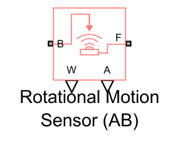

This Simscape schematic shows:

The axis points from left to right, indicated by the two-port blocks showing port B on the left and port F on the right.
Rotational World (AB) block models a stationary point with an angle of theta = 0 deg.
An Inertia (AB) block models a blue disc with an initial Angular velocity of 5 deg/s.
Another Inertia (AB) block models a yellow disc with an initial Angular velocity of 10 deg/s.
Rotational Motion Sensor (AB) blocks measure the angles of the discs.
Initial Relative Angle (AB) blocks set initial angles of the discs. These blocks both have the Relative angle parameter equal to 0 deg.

Step 3: Open the scope and simulate the model when both Initial Relative Angle blocks have Relative angle equal to 0 deg .

open_system('InterpretingAngleFreeDiscs/Disc Angles (deg)');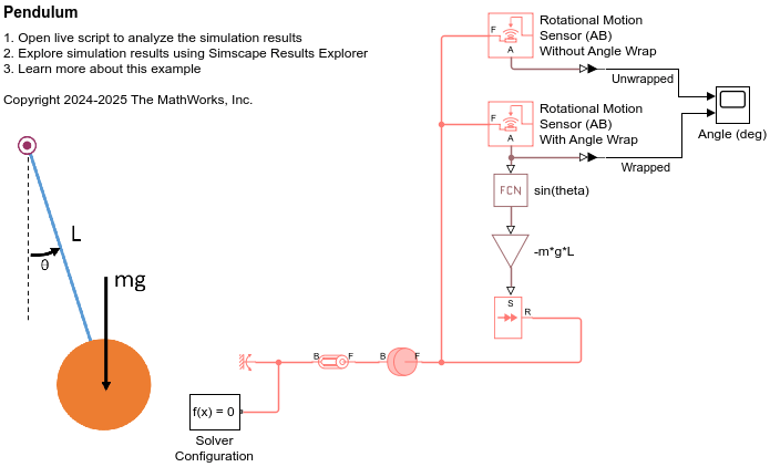

set_param('InterpretingAngleFreeDiscs/Initial Relative Angle (AB) 1', 'theta_rel', '0');
set_param('InterpretingAngleFreeDiscs/Initial Relative Angle (AB) 2', 'theta_rel', '0');
sim('InterpretingAngleFreeDiscs');

The scope shows that both discs start with angles of 0 degrees. The discs move independently of each other after initialization.

Step 4: Adjust the initial angles of the discs.

Open the dialog box of the Initial Relative Angle (AB) 1 block. Change the Relative angle from 0 deg to 60 deg.
Open the dialog box of the Initial Relative Angle (AB) 2 block. Change the Relative angle from 0 deg to -40 deg.

You can alternatively programmatically set the parameter values using these set_param commands instead of using the dialog box.

set_param('InterpretingAngleFreeDiscs/Initial Relative Angle (AB) 1', 'theta_rel', '60');
set_param('InterpretingAngleFreeDiscs/Initial Relative Angle (AB) 2', 'theta_rel', '-40');

Simulate the model.

sim('InterpretingAngleFreeDiscs');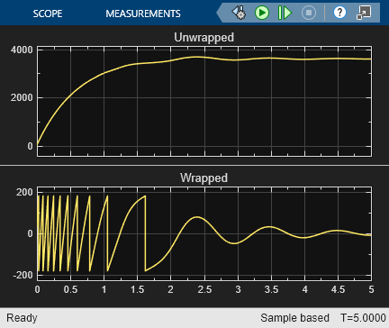

Now, the scope shows that the blue disc starts with an angle of 60 degrees and the yellow disc starts with an angle of 20 degrees, matching the initial conditions shown in the physical view.

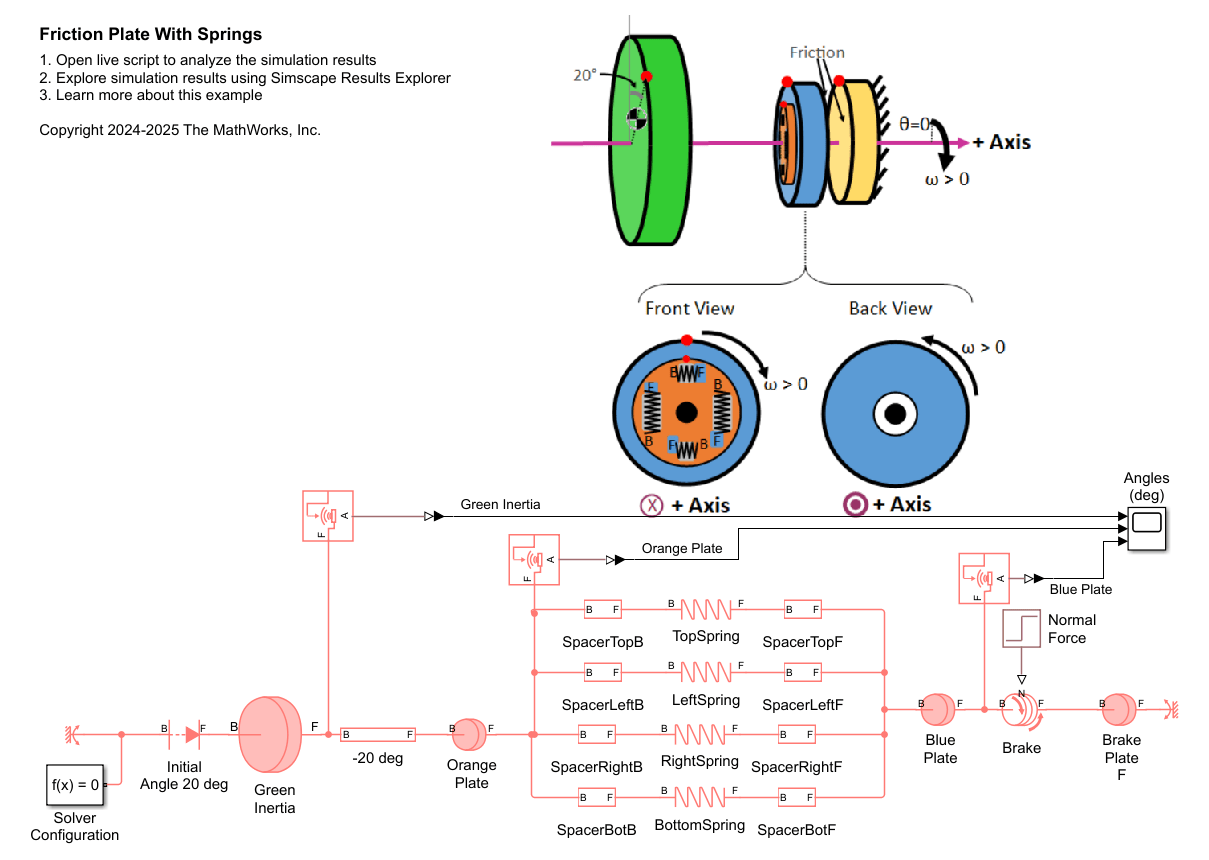
Model of Discs on a Compliant Shaft

This example applies the concepts to model two discs on an elastic shaft. It shows how you can set up and track component angles, even though in this example those angles are not key to the system’s behavior.

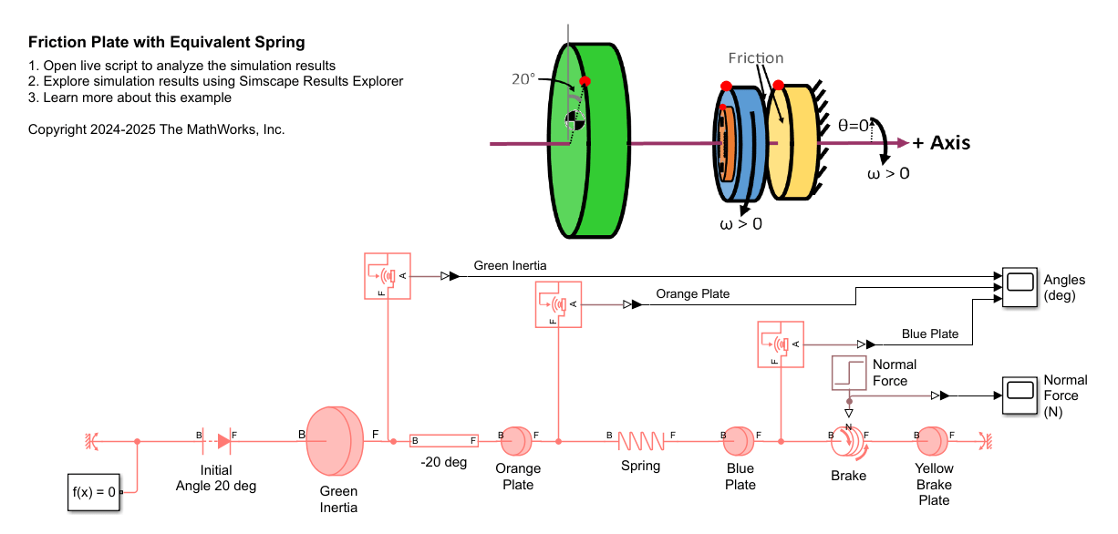
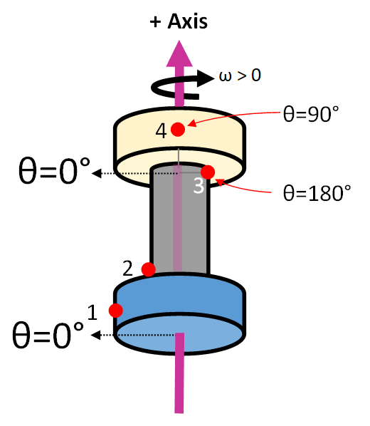
Step 1: Consider a physical system, shown below, with the following characteristics:

The axis points from the blue disc towards the yellow disc, vertically upwards.
The $θ = 0$ direction points to the left in the chosen physical view.
At time = 0 sec, the shaft has no deformation.
At time = 0 sec, angles of the components are:

Point	Description	Initial Angle (deg)
1	Blue disc	0
2	Tracking point on bottom of shaft	0
3	Tracking point on top of shaft	180
4	Yellow Disc	90

Step 2: Open the model.

open_system('InterpretingAngleDiscsOnCompliantShaft');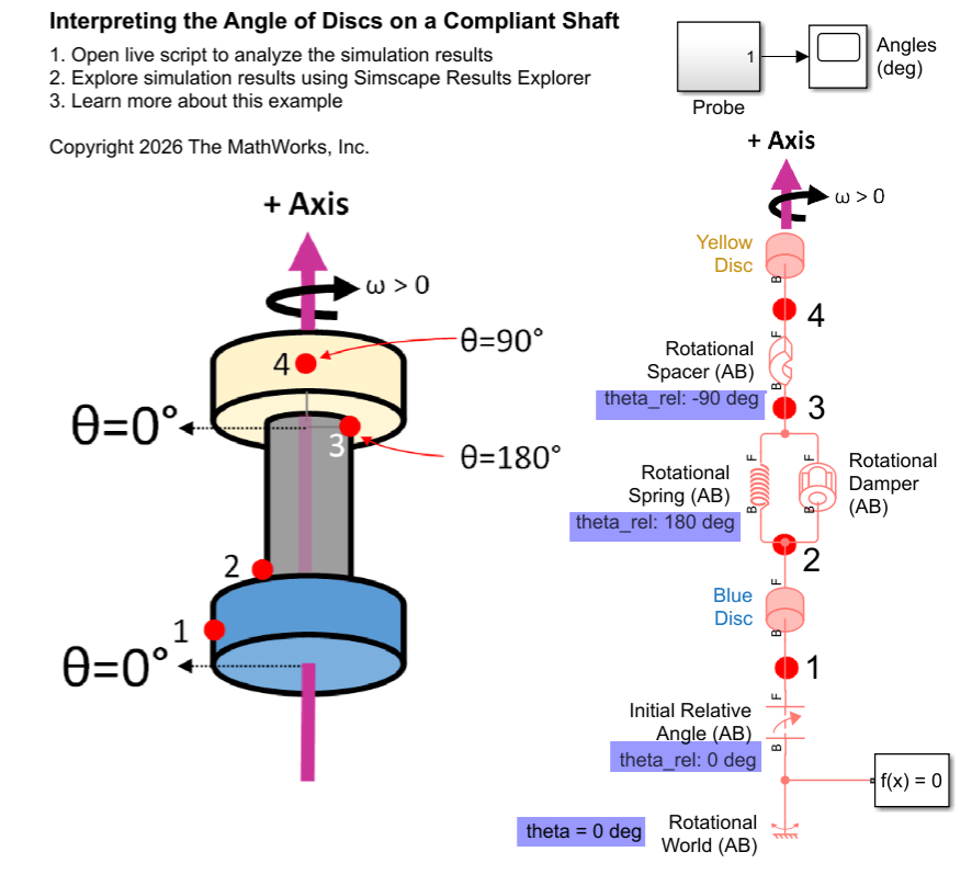

This Simscape schematic shows components and angle settings that mirror the physical view:

The axis points from bottom to top on the canvas, as indicated by the two-port blocks showing port B on the bottom and port F on the top.
Nodes labeled 1 to 4 in the Simscape schematic correspond to tracking points 1 to 4 in the physical view.
Rotational World (AB) block models a stationary point with an angle of 0 deg.
Rotational Spring (AB) and Rotational Damper (AB) in parallel model the compliant shaft.
Initial Relative Angle (AB) block specifies the initial angle of the blue disc relative to the world block.
Rotational Spacer (AB) block shifts the angle between tracking points 3 and 4 on the yellow disc.

The initial angles of the four points are specified by high-priority initial targets of the Relative angle variables in the following blocks:

Initial Relative Angle (AB) with Relative angle of 0 deg.
Rotational Spring (AB) with Relative angle of 180 deg.
Rotational Spacer (AB) with Relative angle of -90 deg.

The purple theta_rel annotation on the Simulink canvas beside each of these blocks displays these initial target values.

To initialize motion, the Blue Disc has an accelerational Torque of 10 N*m.

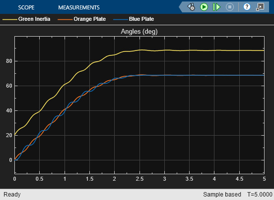
Step 3: Open the scope and simulate the model to view the angles versus time.

Simulate the system and view the angles versus time.

open_system('InterpretingAngleDiscsOnCompliantShaft/Angles (deg)');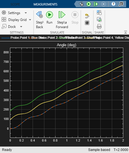

sim('InterpretingAngleDiscsOnCompliantShaft');

At the start of the simulation, blue disc and bottom of the shaft are both at an angle of 0 deg. The yellow disc has an angle of at an angle of angle of 90 deg and the top of the shaft has an angle of 180 deg. During the simulation, the angle between the bottom and top of the shaft varies while the shaft torsionally twists. The angle between the stop of the shaft and yellow disc is fixed to -90 deg, as indicated in the physical view.

Model of a Pendulum and Rotational Motion Sensor (AB) with Angle Wrapping

This model illustrates how to wrap the angle in a Rotational Motion Sensor (AB) block. The pendulum initially has a large rotational velocity so that it revolves around the axis several times before slowing down due to damping.

Open the model.

open_system('InterpretingAnglePendulum');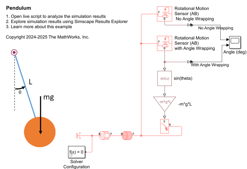

Simulate the model and compare the angles sensed by rotational motion sensors.

open_system('InterpretingAnglePendulum/Angle (deg)');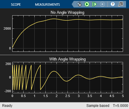

sim('InterpretingAnglePendulum');

At the beginning of the simulation, the pendulum has a high velocity and completes several revolutions around the pivot point. The Rotational Motion Sensor (AB) Wrapped Angle block measures the angle over [-180, 180) degrees. Near the end of the simulation, the damper has slowed down the pendulum so that it undergoes small oscillations about 0 degrees. Choosing a wrap angle of -180 degrees, that is far from the pendulum equilibrium angle, allows the sensor to measure the small rotational oscillations cleanly without angle jumps at the wrap angle.

Summary

Components rotate around an axis.
Specify the axis direction in both the physical view and the schematic.
Place components on the axis in the schematic to represent the physical system.
Align the positive direction of blocks with the positive axis direction.
The Rotational World (AB) block sets the reference frame.
Positive rotational motion follows a right-hand rule around the axis.
Choose a stationary direction for $θ = 0$ .
Choose a tracking point on axisymmetric components. The node logs theta = 0 when the tracking point aligns with the $θ = 0$ direction.
The ports of some two-port blocks can rotate relative to each other.
The ports of other two-port blocks have the same angle as each other.
Use an Initial Relative Angle (AB) block to set an initial angle between two points.
Use a Rotational Spacer (AB) block to set a constant angle between two points.
You can wrap the measured angle of the Rotational Motion Sensor (AB) block to clearly visualize motion that spans a large angle range.