Reduce Computation Costs
Computational cost is a measure of the number and the complexity of tasks that a processor performs per time step during a simulation. Lowering the computational cost of your model increases simulation execution speed and helps you to avoid overruns when you simulate in real time on target hardware.
Data Logging and Monitoring Guidelines
Data logging and monitoring are interactive procedures that consume memory and processing power. One way to reduce computational cost is to reduce the amount of interactive processing that occurs during simulation. Best practices for limiting computational costs while logging and monitoring data are:
Use an outport block only if you need to log data for your analysis via the Simulink® model on your development computer.
Use a scope block only if you need to monitor data during real-time simulation via the Simulink model on your development computer.
If you need to log data or monitor a variable, limit the number or the decimation of data points that you collect whenever your analysis requirements permit you to do so.
Log data only once.
If you use Simscape™ data logging, use local settings to log only the blocks that contain variables that you need for your analysis.
Note
Simscape simulation data logging is not supported for generated code.
Improve Data Logging and Monitoring Efficiency
Examine the configuration of the model and the simulation results to determine if the model is logging and monitoring data efficiently.
To open the model, at the MATLAB® command prompt, enter:
model = 'ssc_pneumatic_rts_zc_redux';
open_system(model)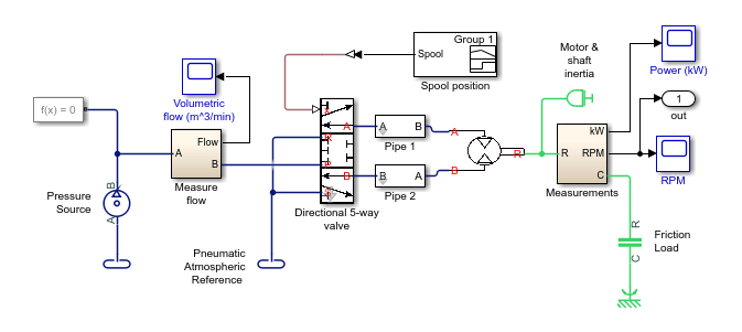
The model contains three scope blocks and one outport block. The Power (kW) scope, RPM scope, and outport block receive data from the Measurements subsystem.
Simulate the model:
sim(model)
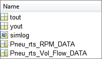
The model logs five variables to the workspace, including a Simscape simulation data logging node.
To determine the source for the
Pneu_rts_RPM_DATA, in the MATLAB workspace, open the structure. Alternately, at the command line, enter:Pneu_rts_RPM_DATA.blockName
ans =

    'ssc_pneumatic_rts_zc_redux/RPM'
The
blockNamevariable shows that the RPM scope logs the data. In the model, the outport that logs data toyoutconnects to the signal between the Measurements subsystem and the RPM scope block.To compare the data that
Pneu_rts_RPM_DATAandyoutlog, plot both data sets to a single figure.h1 = figure; plot(tout,yout) h1; hold on plot(Pneu_rts_RPM_DATA.time,Pneu_rts_RPM_DATA.signals.values,'r--') title('Speed') xlabel('Time (s)') ylabel('Speed (rpm)') h1Leg = legend({'yout','Pneu-rts-RPM-DATA'});

The data is the same, which means that you are logging the same data twice.
To reduce the computational cost for logging or monitoring the speed data via the Simulink model on your development computer during real-time simulation:
If you only need to log the speed data, delete the RPM scope block.
If you need to log and monitor the speed data, delete the outport block.
If you only need to monitor the speed data, delete the outport block and disable data logging for the RPM scope.
If you do not need to log or monitor the speed data via the Simulink model on your development computer during real-time simulation with target hardware, delete both the RPM scope block and the outport block.
If you want to reduce costs by deleting the scope and outport blocks, but you want
to log data while you prepare your model for real-time simulation, configure the
model to log only the data that you need. To do so, use a simlog
node in the MATLAB workspace. For information, see Log Data for Selected Blocks Only.
Additional Methods for Reducing Computational Cost
In addition to reducing the number of logged and monitored signals, you can use these methods for decreasing the number and complexity of tasks that the processor performs per time step during simulation:
Avoid using large images and complex graphics.
Disable unnecessary error and warning diagnostics.
Reconfigure tolerances.
Simplify complex subsystems or replace them with lookup tables.
Linearize nonlinear effects.
Eliminate redundant calculations, for example, multiplication by one.
Reduce the number of differential algebraic equations (DAEs).