Battery State of Charge Estimation using Extremum Seeking Control

Since R2025a

This example shows how to construct a virtual sensor for a battery cell state of charge (SOC) using Extremum Seeking Control (ESC). In this example, you use ESC for parameter estimation instead of controlling the plant. Extremum seeking control provides a unique data-driven approach to construct a virtual sensor, different from all existing techniques. This virtual sensor application showcases the versatility of ESC as a data-driven approach for parameter estimation.

SOC Estimation of Battery Cells

The SOC is the ratio of the released capacity ${\mathit{C}}_{\mathrm{releasable}}$ to the rated capacity ${\mathit{C}}_{\mathrm{rated}}$. Manufacturers provide the value of the rated capacity ${\mathit{C}}_{\mathrm{rated}}$ of each battery but the releasable capacity ${\mathit{C}}_{\mathrm{releasable}}$ is not measurable in

$\mathrm{SOC}=\frac{{\mathit{C}}_{\mathrm{releasable}}}{{\mathit{C}}_{\mathrm{rated}}}$.

State of Charge (SOC) estimation is a key component of a battery management systems (BMS) that ensures the safe and efficient battery operation of a battery. Various traditional techniques are used to estimate SOC, including Kalman Filter, Adaptive Kalman Filter, and Coulomb Counting techniques. For more information, see Estimators​ (Simscape Battery). Since you cannot measure SOC directly from a battery cell, these estimators are virtual sensors that estimate SOC using other measurements such as current and terminal voltage.

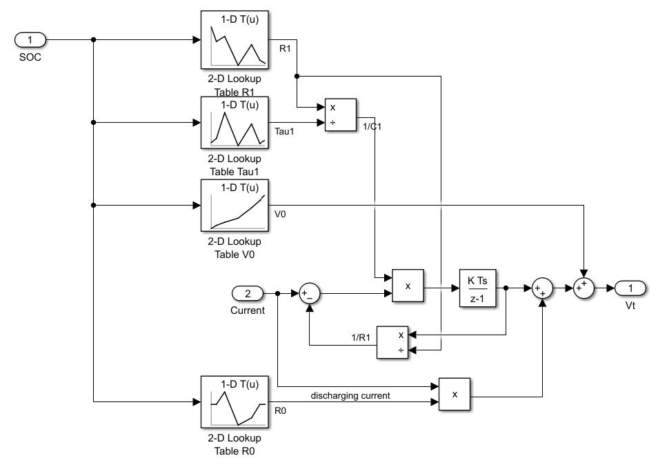
For SOC estimation, a simple one time-constant battery equivalent circuit model is widely used to represent the dynamic behavior of a battery cell. The following figure shows an equivalent circuit with one RC pair:

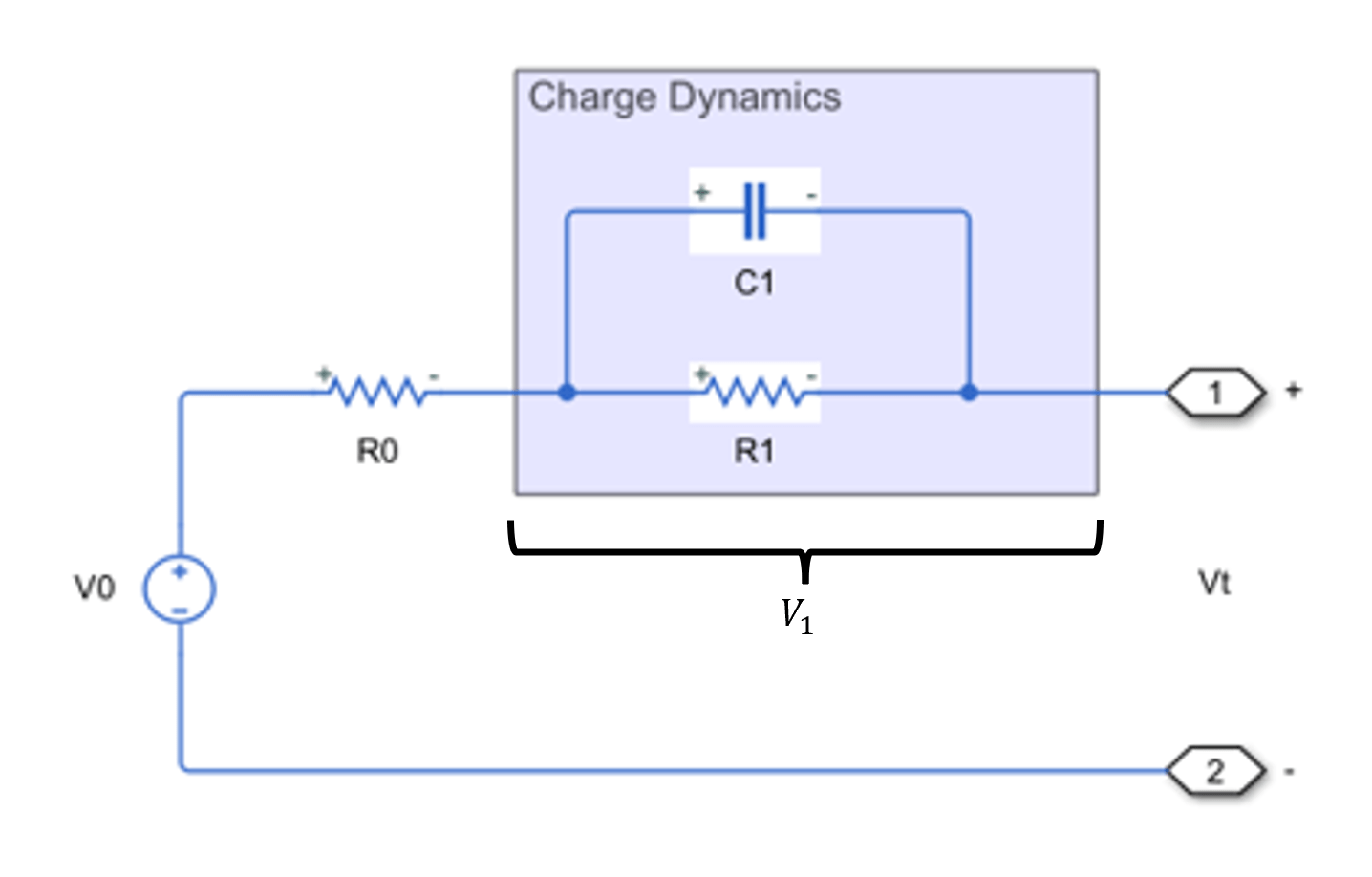
In the equivalent circuit, the relationship between the battery cell's terminal voltage${\mathit{V}}_{\mathit{t}}$ and current $\mathit{i}$ is expressed as:

$${\mathit{V}}_{\mathit{t}}={\mathit{V}}_{\mathit{o}}\left(\mathrm{SOC}\right)-{\mathit{iR}}_0\left(\mathrm{SOC}\right)-{\mathit{V}}_1$$

Here:

• $\mathit{SOC}$ is the state of charge.

• $\mathit{i}$ is the current.

• ${\mathit{V}}_{\mathit{o}}$ is Open-Circuit Voltage.

• ${\mathit{R}}_0$ is the internal resistance.

• ${\mathit{V}}_1$ is the polarization voltage over the RC pair.

Representing the charging/discharging behavior, the polarization voltage ${\mathit{V}}_1$ is governed by the following dynamic equation.

$$\dot{{\mathit{V}}_1}=\frac{\mathit{i}}{{\mathit{C}}_1\left(\mathrm{SOC}\right)}-\frac{{\mathit{V}}_1}{{\mathit{R}}_1\left(\mathrm{SOC}\right)\cdot {\mathit{C}}_1\left(\mathrm{SOC}\right)}=\frac{\mathit{i}}{{\mathit{C}}_1\left(\mathrm{SOC}\right)}-\frac{{\mathit{V}}_1}{{\tau }_1\left(\mathrm{SOC}\right)}$$

Here:

• ${\mathit{R}}_1$ is the polarization resistance.

• ${\mathit{C}}_1$ is the parallel RC capacitance.

• ${\tau }_1$ is the time constant of the RC network.

The virtual sensor uses the algebraic and dynamic equations to estimate the battery cell's SOC level. Within the one time-constant framework, all parameters depend on the SOC level.

Specify Battery Cell Parameters

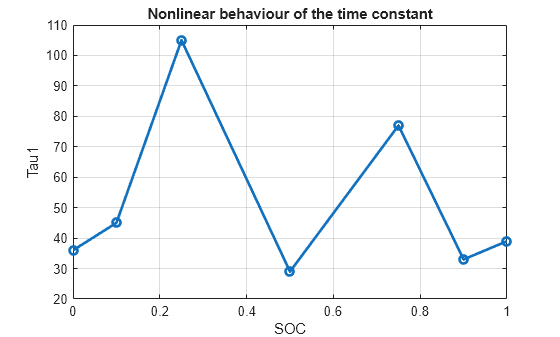
For a realistic battery cell, the ${\mathit{V}}_{\mathit{o}}$, ${\mathit{R}}_{\mathit{o}}$, ${\mathit{R}}_1$ and ${\mathit{C}}_1$ parameters are typically nonlinear with respect to SOC. This nonlinearity in the cell dynamics makes the SOC estimation task more challenging. In this example, you define the cell parameters using the following vectors and implement them through lookup tables.

SOC_vec = [0, .1, .25, .5, .75, .9, 1];                             % SOC values
V0_mat = [3.5057, 3.566, 3.6337, 3.7127, 3.9259, 4.0777, 4.1928];   % Open-circuit voltage V0
R1_mat = [.0029, .0024, .0026, .0016, .0023, .0018, .0017];         % First polarization resistance R1
Tau1_mat = [36, 45, 105, 29, 77, 33, 39];                           % Time constant for the RC network
R0_mat = [.0085, .0085, .0087, .0082, .0083, .0085, .0085];         % Internal resistance R0

For example, plotting the time constant parameter ${\tau }_1$ with respect to the SOC shows obvious nonlinear characteristics. The time constant curve does not follow any monotonicity as SOC changes.

plot(SOC_vec, Tau1_mat, "o-", "LineWidth", 2)
grid on
xlabel("SOC")
ylabel("Tau1")
title("Nonlinear behaviour of the time constant")

Define the initial SOC value for the battery cell plant model.

soc_init = 0.5;

Extremum Seeking Control (ESC) for SOC Estimation

Typically, in ESC, you generate an objective function using some measurable quantity of the system. The ESC algorithm adjusts the other system parameters in order to maximize the objective function.

In a battery cell, the terminal voltage${\mathit{V}}_{\mathit{t}}$ is the measurable quantity. In this example, you use the error between the estimated terminal voltage ${\mathit{V}}_{\mathit{t}\_\mathrm{est}}$ (obtained from the cell model) and the measured terminal voltage ${\mathit{V}}_{\mathit{t}}{\_}_{\mathrm{meas}}$ as our ESC objective function.

$$\mathit{J}=-100*{\left({\mathit{V}}_{\mathit{t}\_\mathrm{est}}-{\mathit{V}}_{\mathit{t}\_\mathrm{meas}}\right)}^2$$

As the terminal voltage depends on the SOC level, the ESC algorithm adapts the SOC values to maximize the cost function to minimize the terminal voltage error. The coefficient 100 in the equation ensures that the estimated SOC tracks the actual value closely. Here the ESC algorithm estimates a system parameter instead of tuning a control parameter like in traditional control problems.

Specify Extremum Seeking Control Parameters

This example uses the Extremum Seeking Control block from SImulink® Control Design™ library, where the following parameters are critical to achieve desired accuracy in the SOC virtual sensor.

Specify the Number of parameters as 1 because you are only estimating the SOC value and set the Sample time of the discrete-time block to 1 sec.

N = 1;       % Number of tuning parameters
Ts = 1;      % Sample time for discrete ESC

Specify the initial guess of the estimated SOC, where Initial condition x0 of 0.8 is different from the actual initial SOC. ESC Algorithm should adapt to a different initial guess quickly as well.

IC = 0.8;    % Initial guess

Based on the default value 1 of Learning rate, typically you start with a small value and gradually increase it while monitoring the algorithm stability and convergence. A learning rate of 2 strikes a good balance between minimizing oscillations and quickly adapting to changes during charging and discharging cycles.

lr = 2;            % Learning Rate

The Forcing frequency omega should be slower than the system dynamics to ensure effective modulation without causing aliasing. However, a frequency that is too low may have little effect on the system. If you analyze the battery equivalent-circuit model Bode response, the response indicates a bandwidth frequency lower than 5 rad/s. Therefore, a forcing frequency of 0.25 rad/s strikes a good balance between minimizing oscillations and allowing adequate time to adjust to changing dynamics.

omega = 0.25;      % Forcing frequency

The SOC estimate varies between 0 and 1. Given the nonlinear nature of cell parameters with respect to SOC, a Modulation amplitude of 0.01 provides a small but noticeable perturbation, making it a good initial guess. Therefore, tuning the Demodulation amplitude around 0.1 typically results in a good SOC estimate, with values stabilizing around 0.07.

mod_amp = 0.01;    % Modulation amplitude
demod_amp = 0.07;  % Demodulation amplitude

Select phase angles for the demodulation signal such that $\cos \left({\varphi }_{\mathrm{mod}}-{\varphi }_{\mathrm{demod}}\right)>0$. Choosing the phase angles to be 0 is suitable for signal correlation in SOC estimation.

mod_phase = 0;     % Modulation phase
demod_phase = 0;   % Demodulation phase

Simulate Battery Cell SOC Estimator

Open the model that implements the ESC algorithm for the battery SOC Estimation problem.

mdl = 'ExtremumSeekingControlSOCEstimator';
open_system(mdl);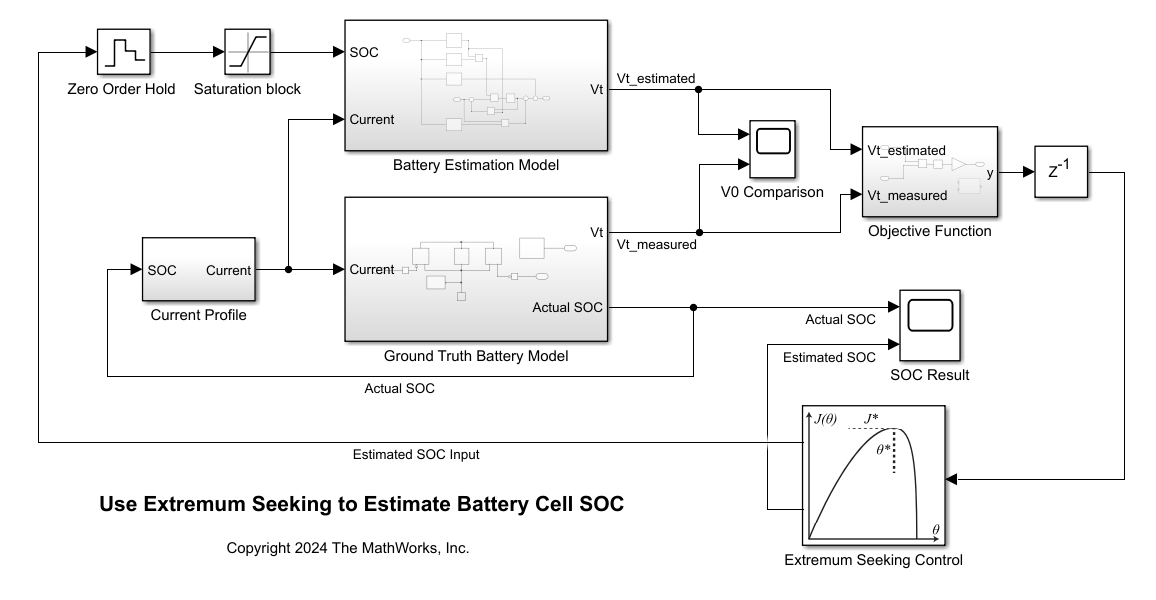

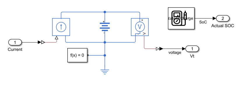
The Battery Estimation Model generates the estimation terminal voltage of the battery cell and the Ground Truth Battery Model is the physical system modeled using Simscape™ Battery™. The physical system model uses a Battery Equivalent Circuit block that does not have any temperature dependence. This ground truth model can be replaced by a plant model with higher fidelity or a real battery cell with sensors providing measurements.

In the estimation model, a linear parameter-varying model is constructed according to the battery cell equivalent circuit. This is a first-order linear system with changing parameters organized using lookup table blocks

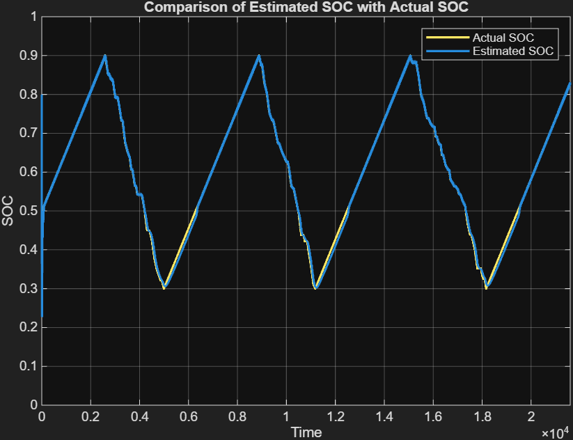
Simulate the model. During the simulation, the Current Profile subsystem simulates the charging and discharging current profile. The model is configured for the cell to charge and discharge for 6 hours.

sim(mdl)

The simulation result shows that the estimated SOC level follows the charging and discharging cycles closely. At the beginning of simulation, the estimated SOC level also converges faster to the truth value compared to the existing SOC estimator blocks.

Close the model.

close_system(mdl,0)

Conclusion

ESC runs faster for SOC estimation problems and requires less computational power compared to more complex methods like the Kalman Filter. The ESC also converges to the actual SOC values faster than the traditional estimation methods. It is computationally efficient, which makes it suitable for real-time applications with limited computational resources. ESC has an adaptive nature, continuously adjusting to changes in system dynamics to maintain optimal performance over time. One of the challenges with using Extremum Seeking Control (ESC) is the difficulty in tuning the ESC parameters. ESC is also more sensitive to measurement noise compared to the Kalman Filter approach.