Measure Frequency Response by Using Complex Data in Stateflow
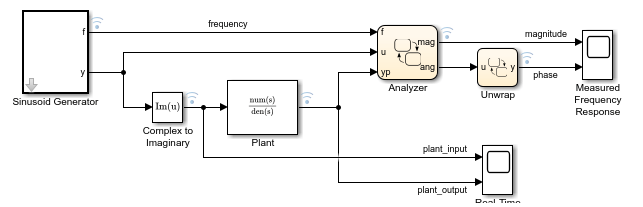
This example shows how to emulate a spectrum analyzer that measures the frequency response of a continuous-time system driven by a complex sinusoidal signal. In this Simulink® model, the Plant block describes a second-order resonant system of the form

with a natural frequency of  (or 150 Hz) and a damping ratio of
  . Because the system is underdamped (
 ), the system has two complex conjugate poles. In a real-world application, replace this block with a subsystem composed of xPC D/A and A/D blocks that measure the response of a device under test (DUT).
The spectrum analyzer consists of these components:
The Sinusoidal Generator block, which produces a complex sinusoidal signal of increasing frequency. Inside the block, a Stateflow® chart uses temporal logic to iterate over a range of frequencies.
The Stateflow chart Analyzer, which calculates the frequency response (magnitude and phase angle) of the system at a specified frequency. The chart registers changes in the frequency by using change detection logic.
The Stateflow chart Unwrap, which processes the measured phase angle and unwraps the result so that there are no sharp jumps between
 and
and  .
.
The spectrum analyzer displays the measured frequency response as a pair of discrete Bode plots.
Generate Sinusoid Signal
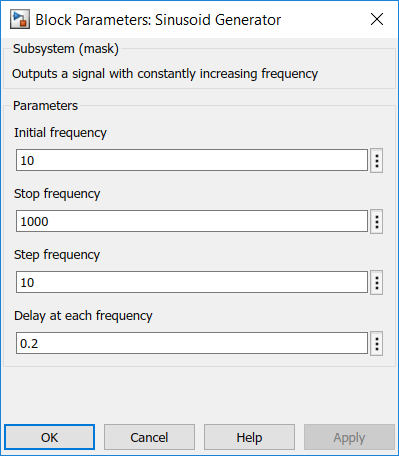
The Sinusoid Generator block has two outputs:
A scalar
fthat represents the current frequency.A complex signal
ythat has a frequency off.
You can control the behavior of the block by modifying its mask dialog box parameters. For example, the default values specify a sinusoidal signal with frequencies between 10Hz and 1000Hz. The block holds each frequency value for 0.2 seconds, and then increments the frequency by a step of 10Hz.
To control the timing of the signal generator, the block contains a Stateflow chart that applies absolute-time temporal logic.
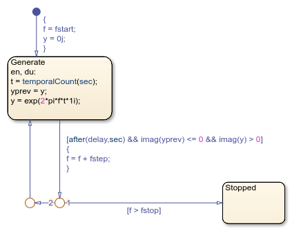
During simulation, the chart goes through these stages:
Initialize Frequency: The default transition sets the signal frequency
fto the value of the parameterfstart. Specify the value offstartin the Sinusoid Generator mask dialog box.Generate Signal: While the
Generatestate is active, the chart produces the complex signaly = exp(2*pi*f*t*1i)based on the frequencyfand the timetsince the last change in frequency. To determine the elapsed time (in seconds) since the state became active, the chart calls the temporal logic operatortemporalCount.Update Frequency: After the
Generatestate is active fordelayseconds, the chart transitions out of the state, increases the frequencyfbyfstep, and returns to theGeneratestate. To determine the timing of the frequency updates, the chart calls the temporal logic operatorafterand checks the sign of the imaginary part of the signal before and after the current time step. The sign checks ensure that the output signal completes a full cycle before the frequency is updated, preventing large changes in the output signal. Specify the values offstepanddelayin the Sinusoid Generator mask dialog box.Stop Simulation: When the frequency
freaches the value of the parameterfstop, the chart transitions to theStoppedstate. The active state outputStoppedtriggers a Stop Simulation (Simulink) block and the simulation ends. Specify the value offstopin the Sinusoid Generator mask dialog box.
Calculate Frequency Response
The Analyzer chart takes the complex signal u and the output yp from the Plant block and computes the magnitude and phase of the plant output.
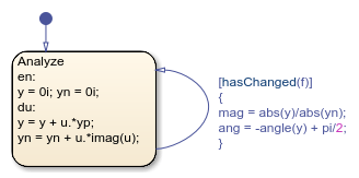
For each frequency value, the chart maintains two running sums:
The sum
yapproximates the integral of the product of the plant outputyp(a real number) and the complex signalu.The sum
ynapproximates the integral of the product of the plant inputimag(u)and the complex signalu. This integral represents the accumulation of a hypothetical plant with a unit transfer function.
To detect a change in frequency, the chart uses the operator hasChanged to guard the self-transition on the state Analyze. When the frequency changes, the actions on this transition compute the magnitude and phase of the plant output by normalizing y with respect to yn.
Unwrap Measured Phase Angle
The Unwrap chart prevents the measured phase angle from changing by more than radians in a single time step.
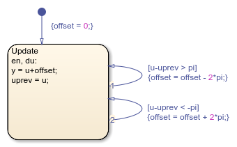
In this chart, the transitions test the change in the input u before computing the new output value y.
If the input increases by more than
radians, the chart offsets the output by  radians.
If the input decreases by more than
radians, the chart offsets the output by  radians.
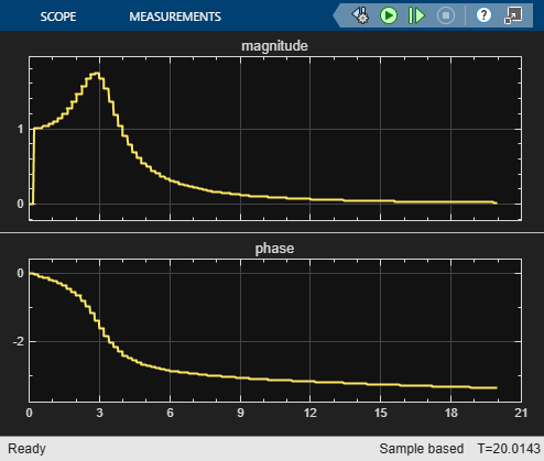
Examine Simulation Results
When you simulate the model, the scope block shows the frequency response of the system (magnitude and phase) as a function of simulation time.
In the magnitude plot, the maximum value at
 indicates the response of the Plant block to a resonant frequency. The peak amplitude is approximately 1.7.
In the phase plot, the angle changes from 0 to
radians. Each complex pole of the system adds  radians to the phase angle.
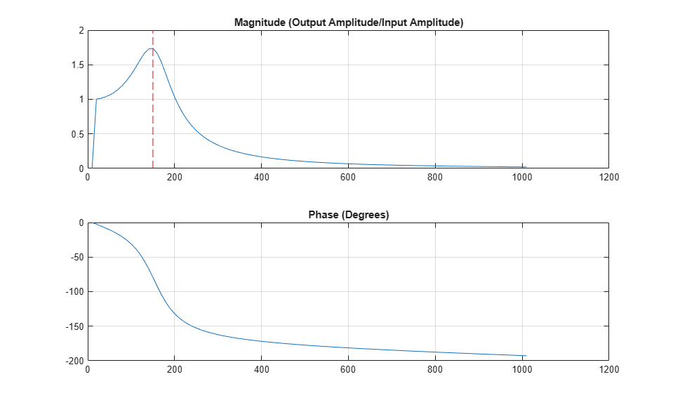
To determine the measured resonant frequency, plot the measured magnitude and phase against the plant input frequency. During simulation, the model saves these values in a signal logging object logsout in the MATLAB® workspace. You can access the logged values by using the get (Simulink)
figure;
subplot(211);
plot(get(logsout,"frequency").Values.Data, ...
    get(logsout,"magnitude").Values.Data);
line([150 150],[0 2],Color="red",LineStyle="--");
grid on;
title("Magnitude (Output Amplitude/Input Amplitude)");
subplot(212);
plot(get(logsout,"frequency").Values.Data, ...
    get(logsout,"phase").Values.Data*180/pi)
grid on;
title("Phase (Degrees)");
The Bode plot shows that the measured resonant frequency is approximately 150Hz, matching the value predicted by the plant dynamics.
See Also
Stop Simulation (Simulink) | after | get (Simulink) | hasChanged | temporalCount