Ground Plane Segmentation of Lidar Data on FPGA
This example shows how to segment organized 3-D lidar point cloud data into ground and nonground parts on FPGA. Ground plane removal is an essential video preprocessing step in lidar applications.
The example model loads a Velodyne® packet capture (PCAP) file from an HDL-32E lidar sensor. The PointCloudReader subsystem uses readFrame to read the input lidar data and separate its location and intensity components. The SegmentGroundFromLidarDataHDL subsystem performs ground plane segmentation in two major steps, Savitzky-Golay smoothing and breadth-first search ground labeling. To observe the segmented lidar data, the PointCloudViewer subsystem uses pcpplayer to create a point cloud visualization. The labeling algorithm assumes the lidar sensor is mounted horizontally so that it observes all ground points closest to the sensor. For more details, see segmentGroundFromLidarData (Computer Vision Toolbox).

Ground Segmentation HDL Subsystem
The input to the HDL subsystem is an organized point cloud, available as a 32-by-2048-by-3 array. The three channels represent the x-, y-, and z- coordinates of the points. The CartesianToSphericalProjection converts these coordinates into a spherical system of range, pitch, and yaw. The SatizskyGolaySmoothing subsystem interpolates any nonfinite outlier values in the lidar measurements. Finally, the BFSGroundLabeling subsystem flood fills the space and labels the connected ground components. To reduce latency and resource use in the flood-fill operation, the model reads the values in an upside-down (row-wise) order.

Savitzky-Golay Interpolate Subsystem
The SavitzkyGolayInterpolate subsystem interpolates the nonfinite values in the range and pitch plane. For range plane interpolation, the subsystem uses the neighbors in the column. If the difference of the neighbors and the current pixel is less than the required rangeThreshold, the mean of the differences is the new interpolated value of the current nonfinite pixel. For pitch plane interpolation, the subsystem uses the left neighbor in the row. Using only the left neighbor optimizes the resources of the design while maintaining performance.

Angle Compute Subsystem
After interpolation, the AngleCompute subsystem computes the angle of inclination from consecutive range values. It takes each column of the range image and calculates the angle. The FloodFill subsystem uses this angle to threshold and label the ground points. Let  and
and  be the range values corresponding to the rows
  and
and  in the range image, then the angle can be computed as,
  . Here,
  and
and  are the vertical angles or pitch values corresponding to the rows and , respectively.

Flood-Fill Subsystem
The BFSGroundLabeling subsystem uses the flood-fill algorithm to segment the ground points. It involves two steps that the SeedsCompute and FloodFill subsystems implement. The seeds act as a starting point for segmenting the ground points. The seedThreshold value is the initial elevation angle of the ground point in the scanning line closest to the lidar sensor. The SeedsCompute subsystem checks if the elevation angle falls below the threshold and marks valid seeds as ground points for every column.
The FloodFill subsystem labels points as ground and nonground points. The flood-fill algorithm accuracy increases with more iterations. However, each iteration requires more hardware resources. This example implements a single iteration that filters more than 90% of the points accurately. The FloodFill subsystem computes the elevation angle difference between one labeled ground point and its four connected neighbors: top, bottom, left, and right. If any of the four neighbors is a ground pixel and the angle difference is less than a specified angleThreshold, then the GroundLabelCompute subsystem labels the point as a ground point.

Simulation and Output
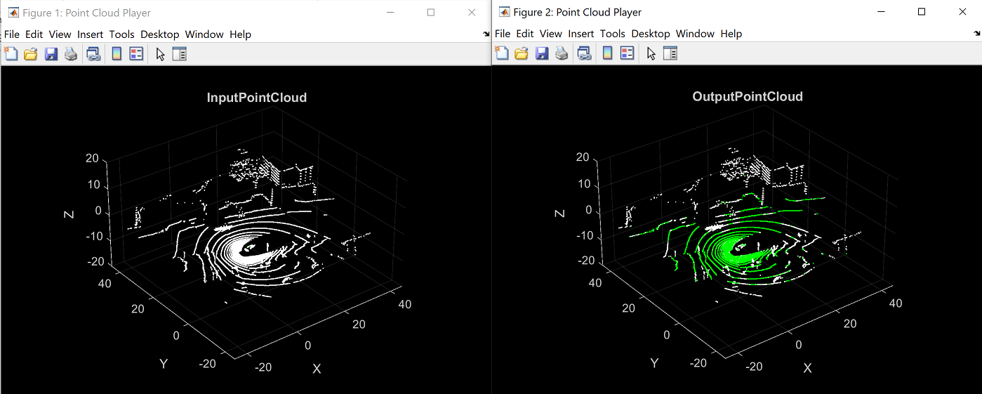
The PointCloudViewer subsystem uses the ground point labels from the point cloud to color all ground points green and nonground points white and plot the resulting lidar point cloud. The plots show the result of ground plane segmentation for the HDL-32E lidar sensor.
Implementation Results
To generate and verify the HDL code from this example, you must have the HDL Coder™ product. To generate the HDL code, use this command.
makehdl('SegmentGroundFromLidarDataHDL/SegmentGroundFromLidarDataHDL')
The generated code was synthesized for an AMD® ZC706 SoC target. The design meets a 150 MHz timing constraint. The table shows the hardware resources for this design.
T =

  5×2 table

    Resource        Usage
    ________    ______________

    DSP48       26 (2.89%)
    Register    39035 (8.93%)
    LUT         33550 (15.35%)
    BRAM        160 (29.36%)
    URAM        0 (0%)
References
[1] Bogoslavskyi, I. "Efficient Online Segmentation for Sparse 3D Laser Scans." Journal of Photogrammetry, Remote Sensing and Geoinformation Science. Vol. 85, Number 1, 2017, pp. 41-52.