Improve Power Amplifier Efficiency Using Crest Factor Reduction

This example shows how to implement crest factor reduction (CFR) technique in orthogonal frequency division multiplexing (OFDM) communication using a Simulink® model. Using this example, you can improve the efficiency of a power amplifier (PA) in an OFDM system with CFR. The Simulink blocks in the example are suitable for HDL code generation.

Crest factor reduction (CFR) is a signal processing technique used primarily in telecommunications to reduce the peak-to-average power ratio (PAPR) of a signal. The crest factor is the ratio of the peak amplitude of a waveform to its average value. A high crest factor indicates that the signal has high peaks relative to its average power, encountered in modern communication methods, such as OFDM systems. These high peaks are undesirable as they increase the PAPR in the system. You can use CFR to reduce the PAPR by limiting the signal peaks to a desired threshold value. By limiting the signal peaks, PA operates in a linear region, improving its efficiency.

There are different methods to implement CFR, such as, clipping, clipping and filtering, peak windowing, peak cancellation, and constrained clipping. This example uses the clipping method to implement CFR.

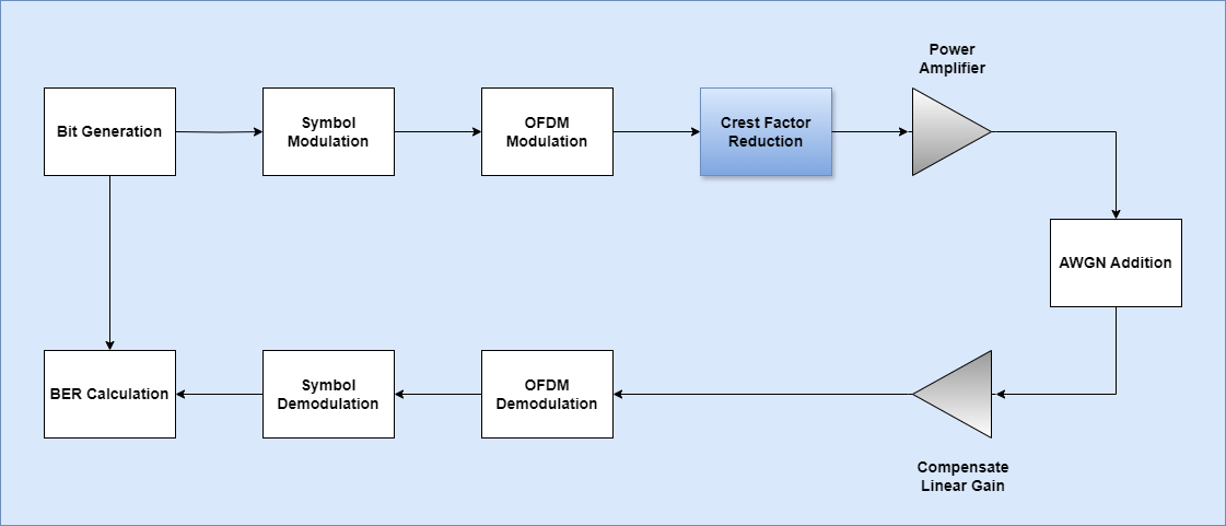
This figure shows the high-level architecture of an OFDM system.

Set Up Input Variables

Specify the values for the input variables to generate an OFDM waveform.

M = 4; % Modulation order for QPSK
Nfft  = 128; % Number of data carriers
Ncp = 32;  % Cyclic prefix length
NSym  = 1000;   % Number of symbols per RE
Nsc = 72; % Number of active subcarriers
scs = 15; % Subcarrier spacing in kHz
SNR = 30; % Signal to Noise power ratio in dB

Generate OFDM Signal

Generate random bits and use the qammod function to get the modulated data symbols. Use the ofdmmod function to generate an OFDM signal and then normalize the signal to unit power.

Nguard = (Nfft/2) - (Nsc/2); % Number of guard subcarriers
ofdmSampleRate = scs*1e3*Nfft; % Time-domain sample rate in Hz
firstSC = Nguard + 1;
nullIndices = [1:(firstSC-1) (firstSC+Nsc):Nfft].';
rng('default');
dataIn = randi([0 M-1],Nsc,NSym); % Generate random data
modSymbols = qammod(dataIn,M,'UnitAveragePower',true); % Symbol modulation
ofdmSymbols = ofdmmod(modSymbols,Nfft,Ncp,nullIndices); % OFDM modulation
% Reshape to create time series
txSignal = reshape(ofdmSymbols, [], 1);
% Normalize signal to unit power
scaleFactor = 1/max(abs(txSignal));
txSignalNorm = txSignal*scaleFactor;

Reduce Crest Factor

To reduce the crest factor, perform the simple clipping operation using this mathematical equation.

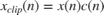, where 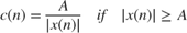and otherwise

To perform clipping, first detect the peaks based on the threshold value. Then, generate a cancellation signal for those peaks and subtract it from the original waveform to obtain the crest factor reduced signal. The threshold is the desired maximum value for the magnitude of the input signal. Specify the threshold value to meet the desired PAPR.

threshold = 0.7; % Peak threshold for peak detection
peaks = abs(txSignalNorm) > threshold;
% Generate the cancellation signal
cancelSignal = zeros(size(txSignalNorm));
for i = 1:length(txSignalNorm)
    if peaks(i)
        cancelSignal(i) = sign(txSignalNorm(i)) * (abs(txSignalNorm(i)) - threshold);
    end
end
% Apply cancellation signal to reduce peaks
reducedSignalML = txSignalNorm - cancelSignal;

Run Crest Factor Reduction Model

Provide the normalized data as an input to the Simulink model. The CrestFactorReduction subsystem in the model performs the crest factor reduction and stores the output data to workspace. Generate input valid signal and run the Simulink model.

integerBits = ceil(log2(max(abs(real(txSignalNorm)))))+2;
stopTime = (length(txSignal)+100)/ofdmSampleRate;
validIn = true(1,length(txSignalNorm));
modelname = "HDLCrestFactorReduction";
open_system(modelname);
out = sim(modelname);
reducedSignalSL = double(out.simOut(out.validOut));

Add Power Amplifier

Use comm.MemorylessNonlinearity System Object™ to apply memoryless nonlinear impairments to the signal. Pass the original signal and CFR signal from MATLAB® and Simulink to the PA. Pass the original signal with a back off of 3 dB to the same PA to evaluate the efficiency of the CFR.

amplifier = comm.MemorylessNonlinearity(Method="Cubic polynomial", ...
    TOISpecification="IPsat",IPsat=30,...
    LinearGain=0,AMPMConversion=30,ReferenceImpedance=50);
origSigAmplified = amplifier(txSignalNorm);
origSigAmplified = origSigAmplified/scaleFactor;
release(amplifier);
cfrSigML = amplifier(reducedSignalML);
cfrSigML = cfrSigML/scaleFactor;
release(amplifier);
cfrSigSL = amplifier(reducedSignalSL);
cfrSigSL = cfrSigSL/scaleFactor;
release(amplifier);

To avoid the nonlinearity introduced by the PA, reduce the input power to the OFDM waveform before the PA. This approach ensures that the PA operates in the linear region. For the configuration used in the example, you can save 3 dB of back-off power by using crest factor reduction.

backOffPower = 3; % Back off power in dB
txSigBackedOff = txSignalNorm/(sqrt((10^(backOffPower/20))));
backedOffSigAmp = amplifier(txSigBackedOff);
backedOffSigAmp = backedOffSigAmp*sqrt(10^(backOffPower/20))/scaleFactor;
release(amplifier);

Perform Demodulation and Compute BER

Add noise to the output of the power amplifier and perform OFDM demodulation. Then, perform symbol demodulation to calculate the demodulated bits, and finally, compute the BER.

% Original signal
rxWaveform = awgn(origSigAmplified,SNR,'measured');
ofdmDemSymbols = ofdmdemod(rxWaveform,Nfft,Ncp,0,nullIndices);
qamDemSymbols = qamdemod(ofdmDemSymbols,M,'UnitAveragePower',true);
bitErrors = sum(sum(bitxor(de2bi(qamDemSymbols),de2bi(dataIn))));
BER_origSig = bitErrors/(log2(M)*numel(dataIn));

% Reduced signal from MATLAB
rxWaveformRedML = awgn(cfrSigML,SNR,'measured');
ofdmDemSymbolsRedML = ofdmdemod(rxWaveformRedML,Nfft,Ncp,0,nullIndices);
qamDemSymbolsRedML = qamdemod(ofdmDemSymbolsRedML,M,'UnitAveragePower',true);
bitErrors = sum(sum(bitxor(de2bi(qamDemSymbolsRedML),de2bi(dataIn))));
BER_cfrSigML = bitErrors/(log2(M)*numel(dataIn));

% Reduced signal from Simulink
rxWaveformRedSL = awgn(cfrSigSL,SNR,'measured');
ofdmDemSymbolsRedSL = ofdmdemod(rxWaveformRedSL,Nfft,Ncp,0,nullIndices);
qamDemSymbolsRedSL = qamdemod(ofdmDemSymbolsRedSL,M,'UnitAveragePower',true);
bitErrors = sum(sum(bitxor(de2bi(qamDemSymbolsRedSL),de2bi(dataIn))));
BER_cfrSigSL = bitErrors/(log2(M)*numel(dataIn));
release(amplifier);

% Original signal with back off
rxSignalBackedOff = awgn(backedOffSigAmp,SNR,'measured');
ofdmDemSymbolsBackOff = ofdmdemod(rxSignalBackedOff,Nfft,Ncp,0,nullIndices);
qamDemSymbolsBackOff = qamdemod(ofdmDemSymbolsBackOff,M,'UnitAveragePower',true);
bitErrors = sum(sum(bitxor(de2bi(qamDemSymbolsBackOff),de2bi(dataIn))));
BER_backedoffSig = bitErrors/(log2(M)*numel(dataIn));

Verify Results

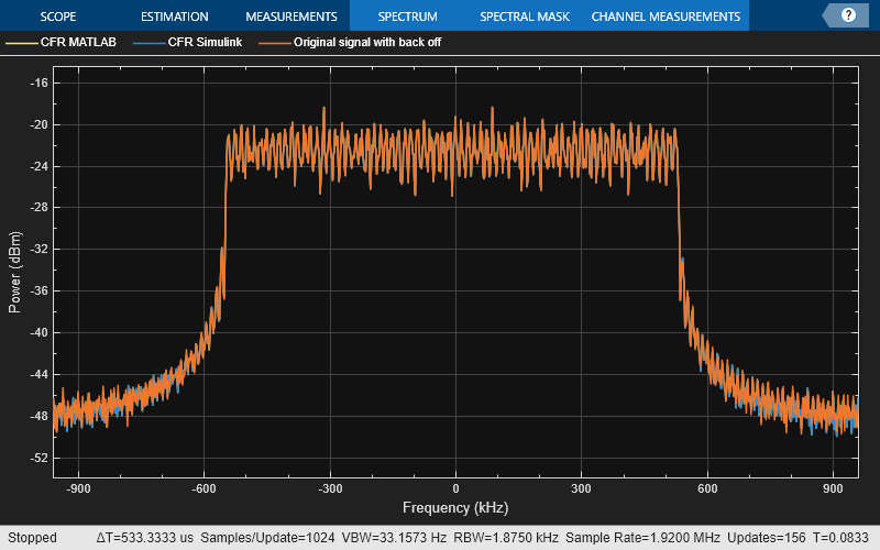
To evaluate the performance of the crest factor reduction algorithm, you can use different metrics, such as, PAPR, bit error rate (BER), and error vector magnitude (EVM).

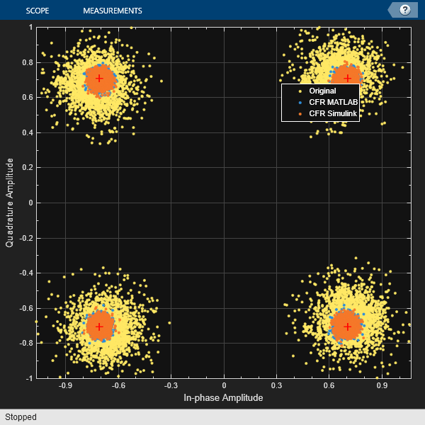
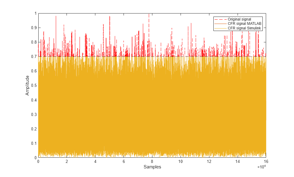
papr_original = max(abs(txSignalNorm).^2) / rms(txSignalNorm.^2);
papr_reducedML = max(abs(reducedSignalML).^2) / rms(reducedSignalML.^2);
papr_reducedSL = max(abs(reducedSignalSL).^2) / rms(reducedSignalSL.^2);

disp(['PAPR of original signal: ', num2str(10*log10(papr_original)), 'dB']);
disp(['PAPR of reduced signal from MATLAB: ', num2str(10*log10(papr_reducedML)), 'dB']);
disp(['PAPR of reduced signal from Simulink: ', num2str(10*log10(papr_reducedSL)), 'dB']);
disp('----------------------');

disp(['Bit error rate for original signal: ', num2str(BER_origSig)]);
disp(['Bit error rate for reduced signal from MATLAB: ', num2str(BER_cfrSigML)]);
disp(['Bit error rate for reduced signal from Simulink: ', num2str(BER_cfrSigSL)]);
disp(['Bit error rate for original signal with back off: ', num2str(BER_backedoffSig)]);
disp('----------------------');

sa = spectrumAnalyzer(SampleRate=ofdmSampleRate,NumInputPorts=3,...
    ChannelNames=["CFR MATLAB","CFR Simulink","Original signal with back off"]);
sa(cfrSigML,cfrSigSL,backedOffSigAmp);
release(sa);

% EVM
evm = comm.EVM;
rmsEVM_origSig = evm(ofdmDemSymbols(:),modSymbols(:));
release(evm);
rmsEVM_cfrSigML = evm(ofdmDemSymbolsRedML(:),modSymbols(:));
release(evm);
rmsEVM_cfrSigSL = evm(ofdmDemSymbolsRedSL(:),modSymbols(:));
release(evm);
rmsEVM_backedoffSig = evm(ofdmDemSymbolsBackOff(:),modSymbols(:));
release(evm);
disp(['RMS EVM for the original signal: ', num2str(rmsEVM_origSig) '%']);
disp(['RMS EVM for the reduced signal from MATLAB: ', num2str(rmsEVM_cfrSigML) '%']);
disp(['RMS EVM for the reduced signal from Simulink: ', num2str(rmsEVM_cfrSigSL) '%']);
disp(['RMS EVM for the original signal with back off : ', num2str(rmsEVM_backedoffSig) '%']);
disp('----------------------');

% Plot constellation
refConst = qammod(0:M-1,M,'UnitAveragePower',true);
axisLimits = [-1 1];
constdiag = comm.ConstellationDiagram(NumInputPorts=3, ...
    ChannelNames=["Original" "CFR MATLAB" "CFR Simulink"],ShowLegend=true, ...
    ReferenceConstellation=refConst, ...
    XLimits=axisLimits,YLimits=axisLimits);
constdiag(ofdmDemSymbols(:),ofdmDemSymbolsRedML(:),ofdmDemSymbolsRedSL(:));
release(constdiag);

% Plot original signal
figure;subplot(3,1,1);
plot(abs(txSignalNorm));
title('Original Signal with High Peaks');
xlabel('Samples');
ylabel('Amplitude');

% Plot cancellation signal
subplot(3,1,2);
plot(abs(cancelSignal));
title('Cancellation Signal');
xlabel('Samples');
ylabel('Amplitude');

% Plot peak-reduced signal
subplot(3,1,3);
plot(abs(reducedSignalML));
title('Signal After Clipping');
xlabel('Samples');
ylabel('Amplitude');

figure;
plot(abs(txSignalNorm),'--r');
hold on;
plot(abs(reducedSignalML));
hold on;
plot(abs(reducedSignalSL));
hold on;
yline(threshold,'--')
xlabel('Samples');
ylabel('Amplitude');
legend('Original signal','CFR signal MATLAB','CFR signal Simulink');

PAPR of original signal: 9.1723dB
PAPR of reduced signal from MATLAB: 6.1217dB
PAPR of reduced signal from Simulink: 6.123dB
----------------------
Bit error rate for original signal: 0
Bit error rate for reduced signal from MATLAB: 0
Bit error rate for reduced signal from Simulink: 0
Bit error rate for original signal with back off: 0
----------------------
RMS EVM for the original signal: 5.8066%
RMS EVM for the reduced signal from MATLAB: 2.6671%
RMS EVM for the reduced signal from Simulink: 2.6706%
RMS EVM for the original signal with back off : 2.6991%
----------------------

Generate HDL Code

To generate the HDL code for this example, you must have the HDL Coder™ product. Use the makehdl and makehdltb commands to generate HDL code and an HDL test bench for the CrestFactorReduction subsystem.

The resulting HDL code was synthesized for a Xilinx® Zynq® UltraScale+ RFSoC ZCU111 evaluation board. The table shows the post place and route resource utilization results. The design meets timing with a clock frequency of 500 MHz.

T = table(...
    categorical({'CLB Registers'; 'CLB LUTs'; 'BRAMB'; 'DSP'}),...
    [3631; 3131; 0; 4],...
    'VariableNames',{'Resource','Crest Factor Reduction'});
disp(T);

      Resource       Crest Factor Reduction
    _____________    ______________________

    CLB Registers             3631         
    CLB LUTs                  3131         
    BRAMB                        0         
    DSP                          4