Using this library one can derive differential equations for any dynamic systems and solve response of the system for a given conditions.
https://github.com/Mansourt/Matlab_Euler-Lagrange_Library_for_Deriving_Equations_of_Dynamic_Systems
Ahora está siguiendo esta publicación
- Verá actualizaciones en las notificaciones de contenido en seguimiento.
- Podrá recibir correos electrónicos, en función de las preferencias de comunicación que haya establecido.
Using the above library, one can derive differential equations for any dynamic systems and solve response of the system for a given conditions.
Functionality of the library has been illustrated by the following examples:
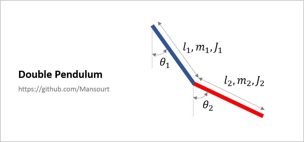
- Double Pendulum
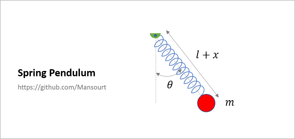
- Spring Pendulum
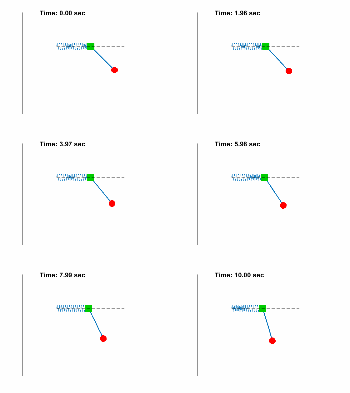
- Pendulum with Spring-loaded support
- Double Pendulum with free support
- Double Spring Pendulum
- Coupled Pendulum
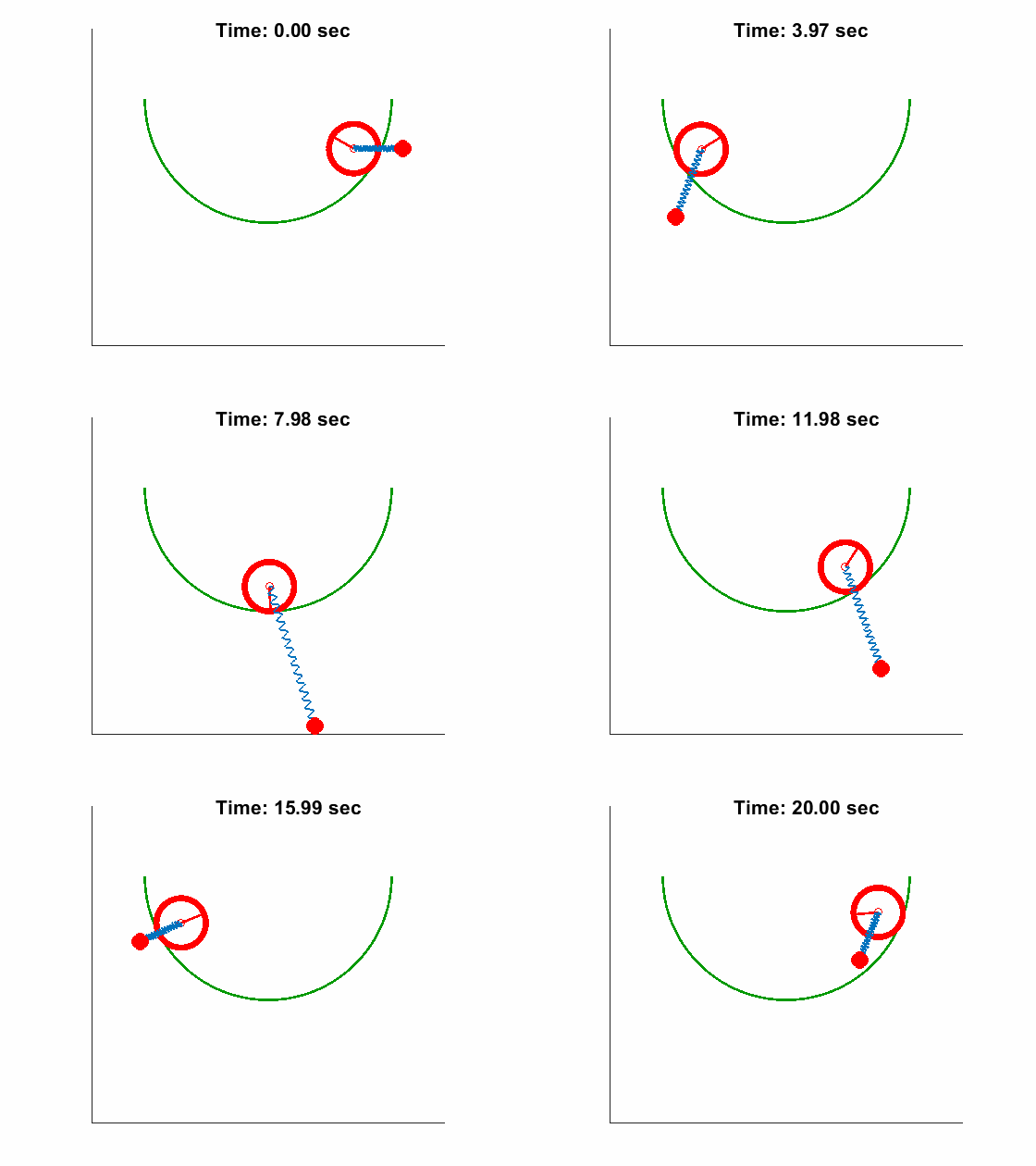
- Spring Pendulum with Rolling base inside a semicircle
Problem Definition:
|
How to solve:
Just run the EVAL1.m to derive equations and solve intial condition problem:
syms th1 th2  Dth1 Dth2
syms l1 l2 m1 m2 J1 J2  g t

%% Kinetic and Potential Energy
T1 = 1/2*J1*Dth1^2 + 1/2*m1*(l1/2*Dth1)^2;

Vc2_x = l1*Dth1*cos(th1) + l2/2*(Dth2)*cos(th2);
Vc2_y = l1*Dth1*sin(th1) + l2/2*(Dth2)*sin(th2);
Vc2 = sqrt(Vc2_x^2 + Vc2_y^2);

T2 = 1/2*J2*(Dth2)^2 + 1/2*m2*Vc2^2;

T = T1 + T2;

V1 = m1*g*l1/2 * (1-cos(th1));
V2 = m2*g*(l1*(1-cos(th1)) + l2/2*(1-cos(th2)));
V = V1 + V2;

L = T - V;
%%
q  = [th1, th2];
Dq = [Dth1, Dth2];
tt = linspace(0,5,500);
Eq = LagrangeDynamicEqDeriver(L, q, Dq);
[SS, xx] = DynamicEqSolver(Eq, q, Dq, [l1 l2 m1 m2 J1 J2 g],...
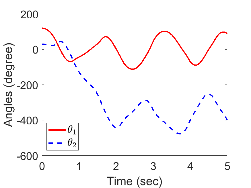
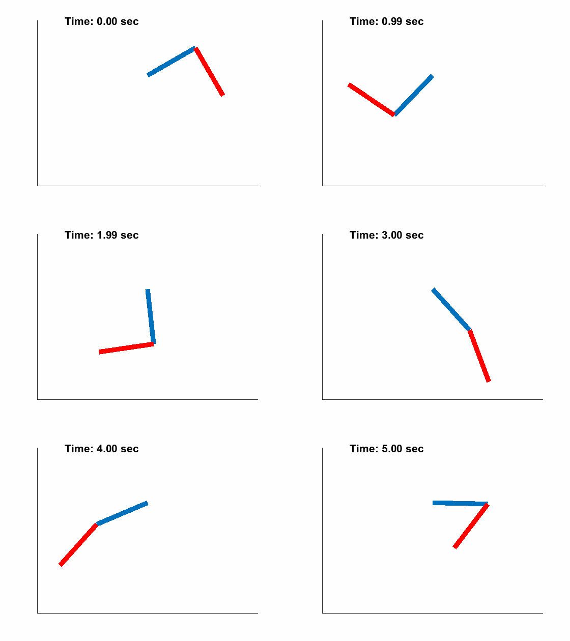
[0.5, 0.5, 1, 5, 0.2, 0.5, 9.81], tt, [120,30,0,0]/180*pi);| Anlges of double pendulum: | Animated Response: |
|---|---|
|
|
Problem Definition:
|
How to solve:
Just run the EVAL2.m to derive equations and solve intial condition problem:
syms th Dth x Dx
syms m l k g t

%% Kinetic and Potential Energy
T = 1/2*m*(Dx^2 + (l + x)^2*Dth^2);
V = -m*g*(l+x)*cos(th) + 1/2*k*x^2;

L = T - V;
%% Derive Equations
q = [th, x]; Dq = [Dth, Dx];
Eq = LagrangeDynamicEqDeriver(L, q, Dq);

%% Solve Equations

tt = linspace(0,10,300);
[SS, xx] = DynamicEqSolver(Eq, q, Dq, [m l k g],...
[1 1 10 9.81], tt, [45/180*pi,0.1, 0, 0]);| Angle and length of spring pendulum: | Animated Response: |
|---|---|
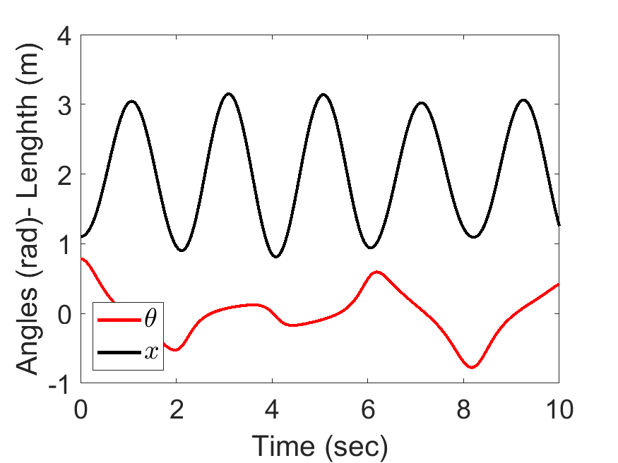
|
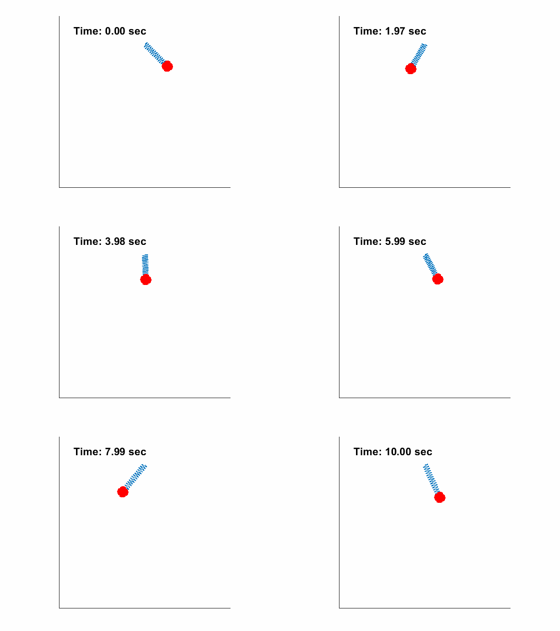
|
Problem Definition:
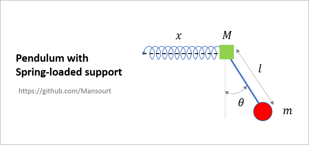
|
How to solve:
Just run the EVAL3.m to derive equations and solve intial condition problem:
syms th Dth x Dx
syms M m l k g

%% Kinetic and Potential Energy
Vx2 = (Dx + l*Dth*cos(th))^2 + (l*Dth*sin(th))^2;
T   = 1/2*m*Vx2 + 1/2*M*Dx^2;

V = m*g*l*(1-cos(th)) + 1/2*k*x^2;

L = T - V;
%% Derive Equations
q = [th, x]; Dq = [Dth, Dx];
Eq = LagrangeDynamicEqDeriver(L, q, Dq);

%% Solve Equations

tt = linspace(0,10,200);
[SS, xx] = DynamicEqSolver(Eq, q, Dq, [M m l k g],...
[2, 1, 0.5, 50, 9.81], tt, [45/180*pi,0, 0, 0]);| Slider Position and Pendulum Anlge: | Animated Response: |
|---|---|
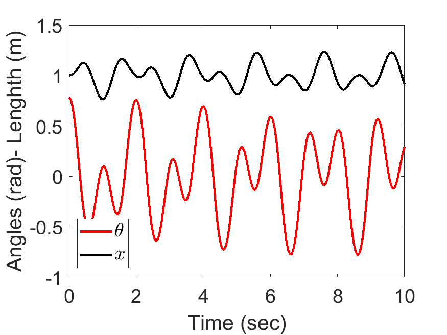
|
|
Problem Definition:
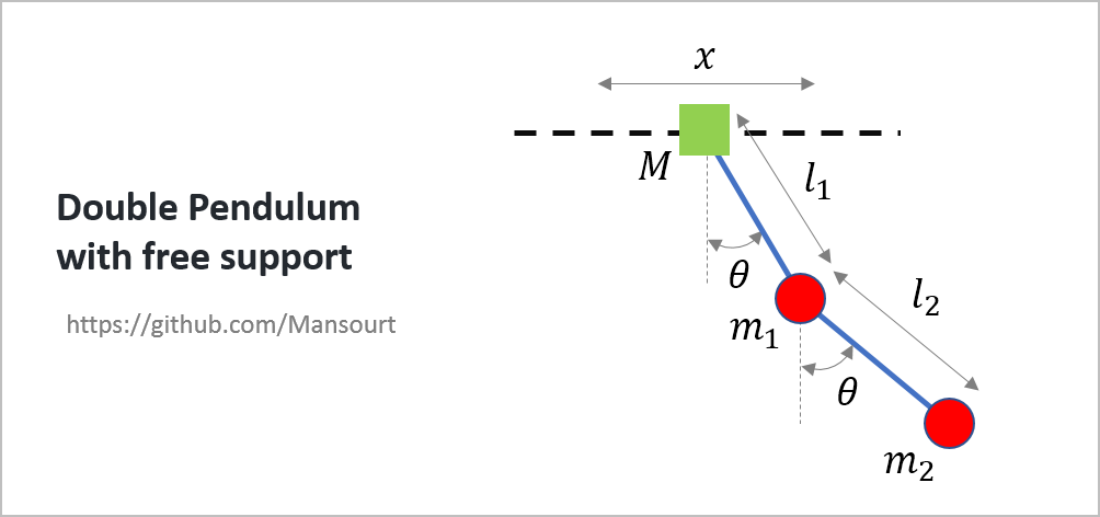
|
How to solve:
Just run the EVAL4.m to derive equations and solve intial condition problem:
syms x th1 th2 Dx Dth1 Dth2
syms M m1 m2 l1 l2 g

%% Kinetic and Potential Energy
v1x = l1*Dth1*cos(th1) + Dx;
v1y = l1*Dth1*sin(th1);

v2x = l1*Dth1*cos(th1) + l2*Dth2*cos(th2) + Dx;
v2y = l1*Dth1*sin(th1) + l2*Dth2*sin(th2);

v1t = v1x^2 + v1y^2;
v2t = v2x^2 + v2y^2;

T = 1/2*M*Dx^2 + 1/2*m1*v1t + 1/2*m2*v2t;

V1 = m1*g*l1*(1-cos(th1));
V2 = m2*g*(l1*(1-cos(th1))+l2*(1-cos(th2)));
V = V1 + V2;

L = T - V;
%%
q  = [x, th1, th2];
Dq = [Dx, Dth1, Dth2];
tt = linspace(0,25,500);
Eq = LagrangeDynamicEqDeriver(L, q, Dq);
[SS, xx] = DynamicEqSolver(Eq, q, Dq, [M m1 m2 l1 l2 g],...
                           [0.5, 0.5, 2, 1, 1, 9.81], tt, [0, pi/3, 2*pi/3, 0, 0, 0]);
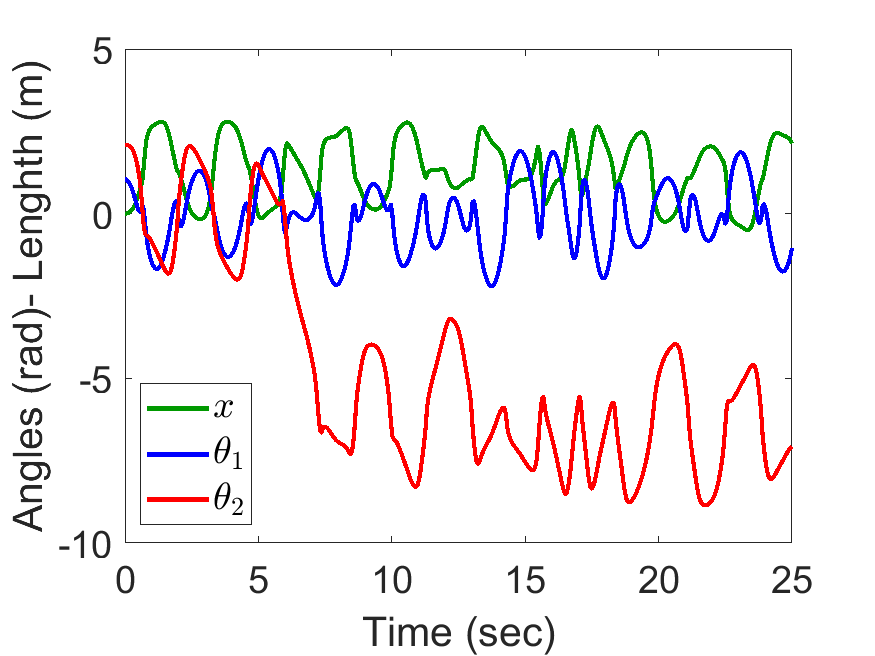
Slider Position, Pendulum Anlges:
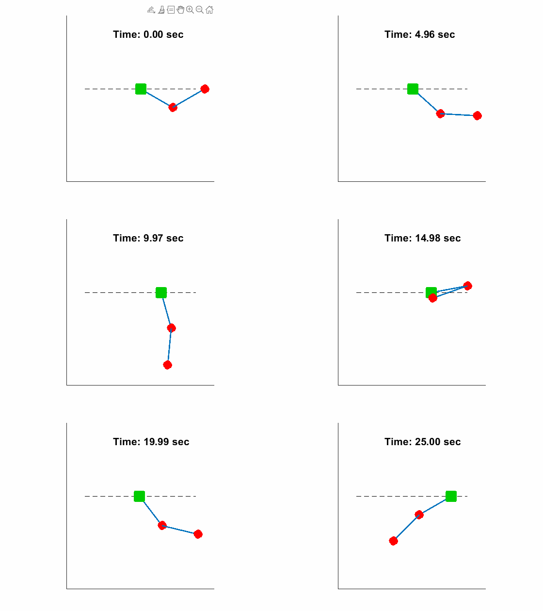
| Slider Position, Pendulum Anlges: | Animated Response: |
|---|---|
|
|
Problem Definition:
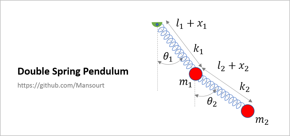
|
How to solve:
Just run the EVAL5.m to derive equations and solve intial condition problem:
syms x1 x2 th1 th2 Dx1 Dx2 Dth1 Dth2
syms k1 k2 m1 m2 l1 l2 g

%% Kinetic and Potential Energy

v1x = Dx1*sin(th1) + (l1 + x1)*Dth1*cos(th1);
v1y = Dx1*cos(th1) - (l1 + x1)*Dth1*sin(th1);

v2x = Dx1*sin(th1) + (l1 + x1)*Dth1*cos(th1) + Dx2*sin(th2) + (l2 + x2)*Dth2*cos(th2);
v2y = Dx1*cos(th1) - (l1 + x1)*Dth1*sin(th1) + Dx2*cos(th2) - (l2 + x2)*Dth2*sin(th2);

v1t = v1x^2 + v1y^2;
v2t = v2x^2 + v2y^2;

T = 1/2*m1*v1t + 1/2*m2*v2t;

V1 = -m1*g*((l1 + x1)*cos(th1)) + 1/2*k1*x1^2;
V2 = -m2*g*((l1 + x1)*cos(th1) + (l2 + x2)*cos(th2)) + 1/2*k2*x2^2;
V = V1 + V2;

L = T - V;
%%
q  = [x1, x2, th1, th2];
Dq = [Dx1, Dx2, Dth1, Dth2];
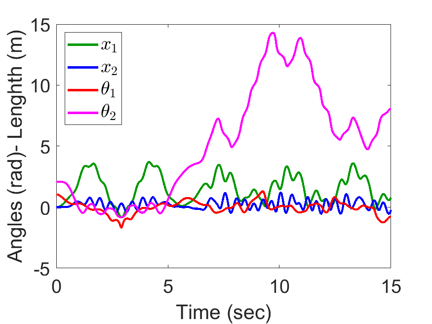
tt = linspace(0, 15, 500);
Eq = LagrangeDynamicEqDeriver(L, q, Dq);
[SS, xx] = DynamicEqSolver(Eq, q, Dq, [k1 k2 m1 m2 l1 l2 g],...
                           [20, 100, 1, 2, 1, 1, 9.81], tt, [0, 0, pi/3, 2*pi/3, 0, 0, 0, 0]);
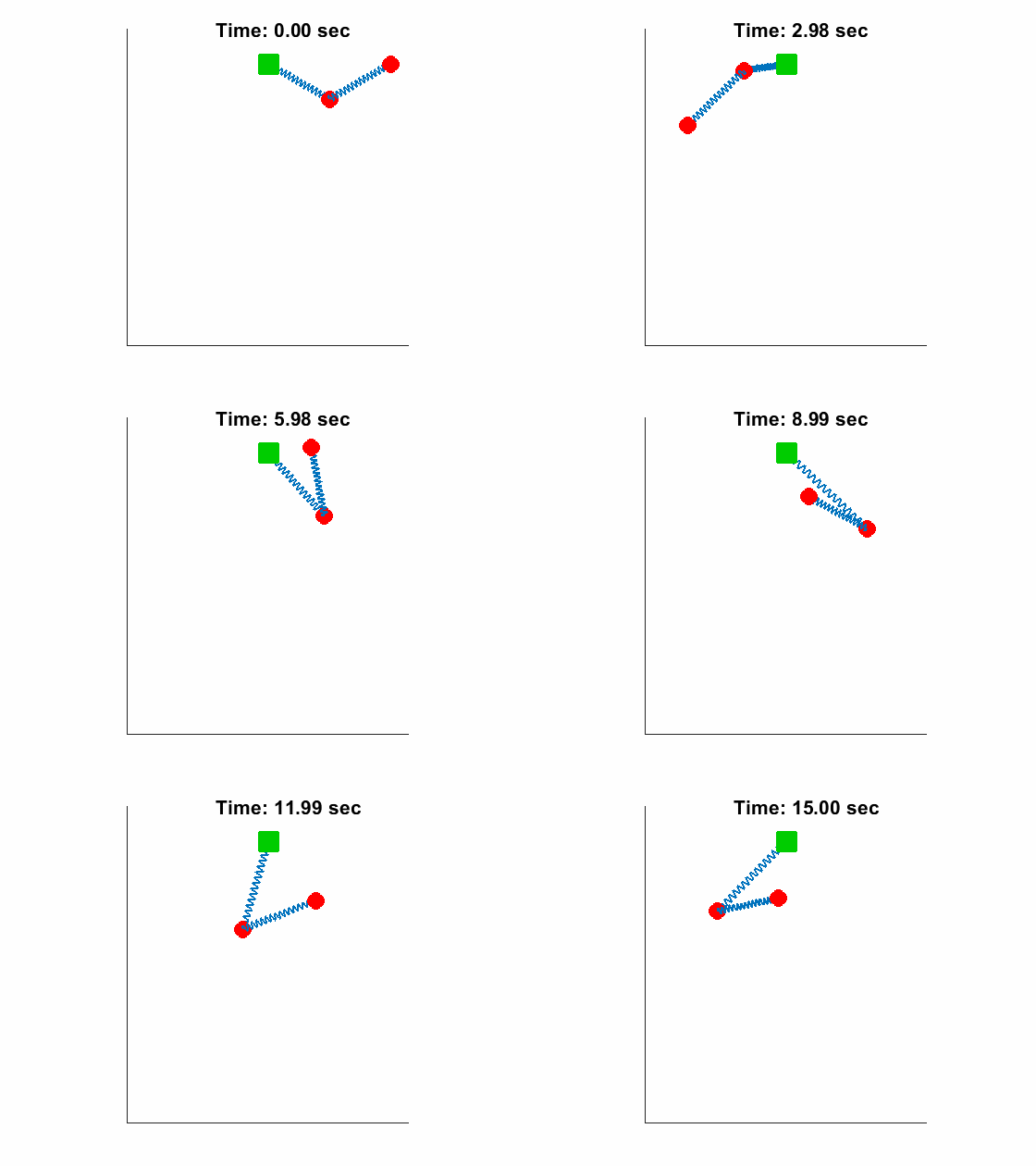
Slider Position, Pendulum Anlges:
| Angle and length of spring pendulum: | Animated Response: |
|---|---|
|
|
Problem Definition:
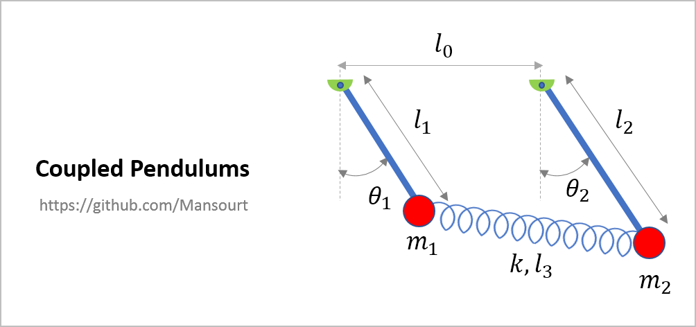
|
How to solve:
Just run the EVAL6.m to derive equations and solve intial condition problem:
syms th1 th2 Dth1 Dth2
syms k m1 m2 l0 l1 l2 l3 g

%% Kinetic and Potential Energy

v1x = l1*Dth1*cos(th1) ;
v1y = -l1*Dth1*sin(th1);

v2x = l2*Dth2*cos(th2) ;
v2y = -l2*Dth2*sin(th2);

v1t = v1x^2 + v1y^2;
v2t = v2x^2 + v2y^2;

T = 1/2*m1*v1t + 1/2*m2*v2t;

dXX = l0 + l2*sin(th2) - l1*sin(th1);
dYY = l1*cos(th1) - l2*cos(th2);
dx = (dXX^2 + dYY^2)^0.5 - l3;

V1 = -m1*g*(l1*cos(th1)) + 1/2*k*dx^2;
V2 = -m2*g*(l2*cos(th2));
V = V1 + V2;

L = T - V;
%%
q  = [th1, th2];
Dq = [Dth1, Dth2];
tt = linspace(0, 20, 500);
Eq = LagrangeDynamicEqDeriver(L, q, Dq);
l0n = 2; l1n = 1; l2n = 1.5; l3n = 2;
[SS, xx] = DynamicEqSolver(Eq, q, Dq, [k m1 m2 l0 l1 l2 l3 g],...
                           [20,1,3, l0n, l1n, l2n, l3n, 9.81], tt, [pi/6, pi/2.5, 0, 0]);
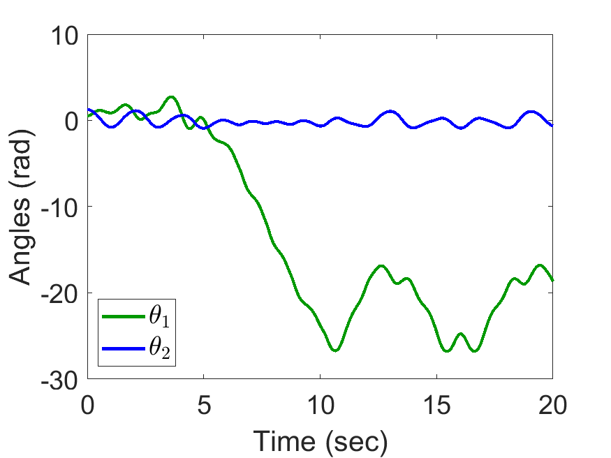
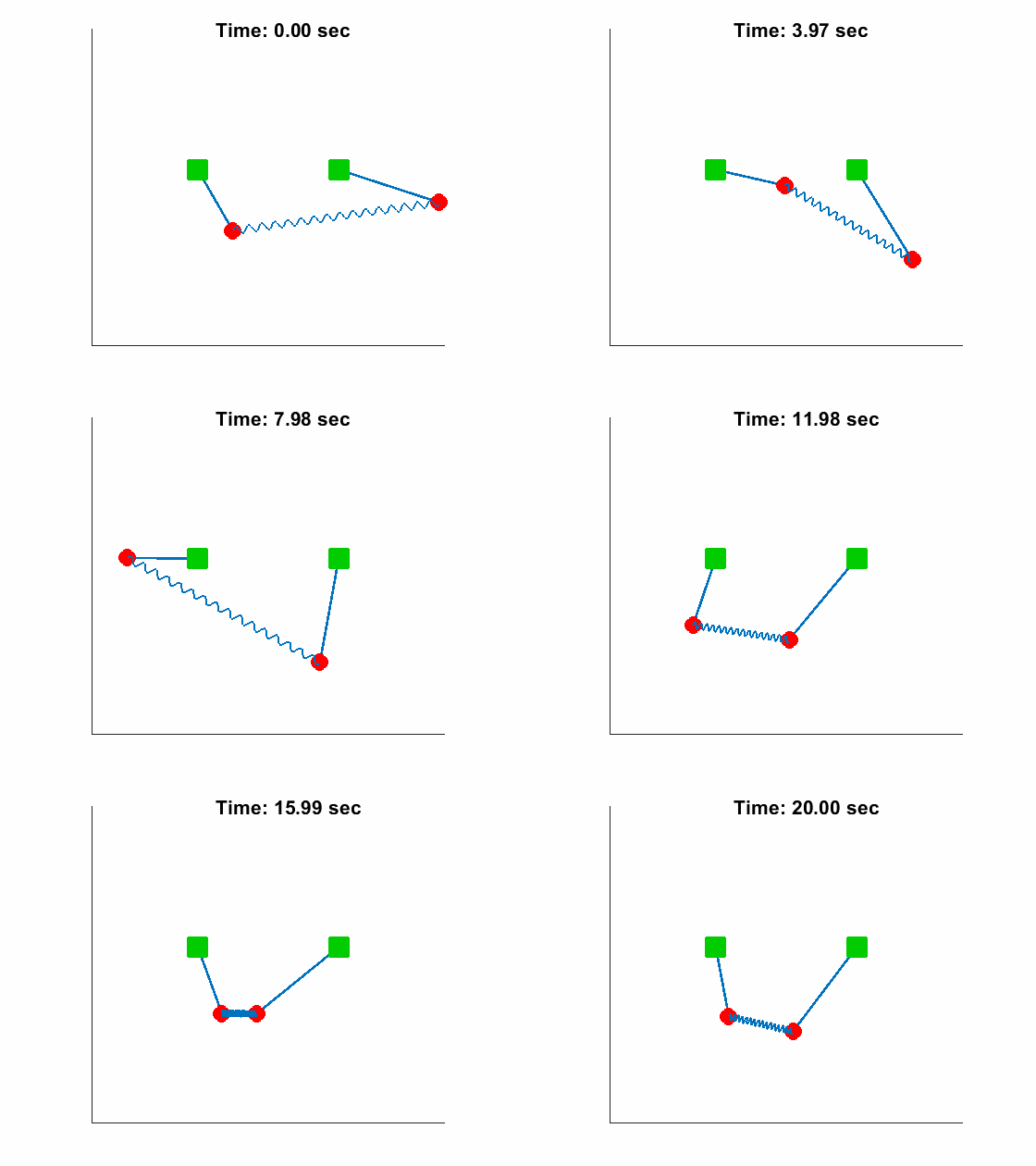
Slider Position, Pendulum Anlges:
| Angles of coupled pendulum: | Animated Response: |
|---|---|
|
|
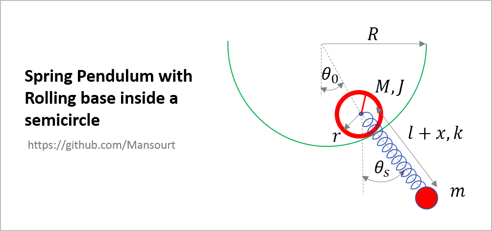
Problem Definition:
|
How to solve:
Just run the EVAL7.m to derive equations and solve intial condition problem:
syms th0 ths x Dth0 Dths Dx
syms R r M J m k l g

%% Kinetic and Potential Energy

VoM = (R-r)*[cos(th0), sin(th0)];
Wd  = -(R-r)*Dth0/r;

Vm = (R-r)*Dth0*[cos(th0), sin(th0)] + (l+x)*Dths*[cos(ths), sin(ths)] + Dx*[sin(ths), -cos(ths)];

yM = -(R-r)*cos(th0);
ym = yM - (l+x)*cos(ths);

T = 1/2*M*(VoM*VoM.') + 1/2*m*(Vm*Vm.') + 1/2*J*Wd^2;

V = M*g*yM + m*g*ym + 1/2*k*x^2;

L = T - V;
%%
q  = [th0, ths, x];
Dq = [Dth0, Dths, Dx];
tt = linspace(0, 20, 500);
Eq = LagrangeDynamicEqDeriver(L, q, Dq);
R0 = 5; r0 = 1; l0 = 2;
[SS, xx] = DynamicEqSolver(Eq, q, Dq, [R r M J m k l g],...
                           [R0, r0, 1, 2, 3, 30, l0, 9.81], tt, [pi/3, pi/2, 0, 0, 0, 0]);
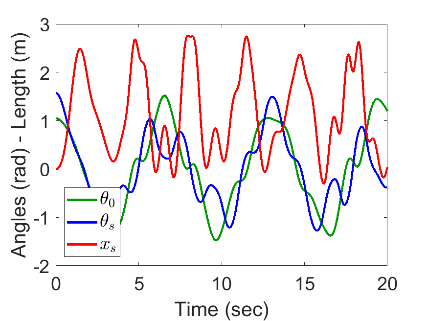
Slider Position, Pendulum Anlges:
| Angles of spring length: | Animated Response: |
|---|---|
|
|
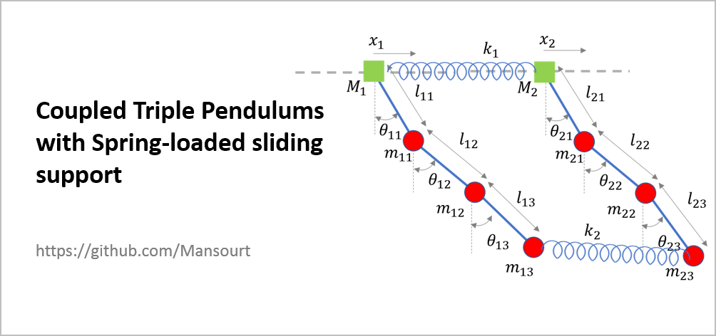
Problem Definition:
|
The simulation results are based on the following Values:
% List of Parameter Values
Plist1 = [M1 m11 m12 m13 l11 l12 l13];
Pval1  = [4, 2, 1,1, 1, 1,1];
Plist2 = [M2 m21 m22 m23 l21 l22 l23];
Pval2  = [8, 2, 1,1, 1, 1,1];

Plist3 = [g l0 ls1 ls2 k1 k2];
Pval3  = [9.8, 1, 1,1, 100,50];

% Initial Conditions
x01  = [0,pi/6,2*pi/6,4*pi/5];
Dx01 = zeros(1,4);
x02  = [0.5,pi/4,2*pi/4,5*pi/8];
Dx02 = zeros(1,4);
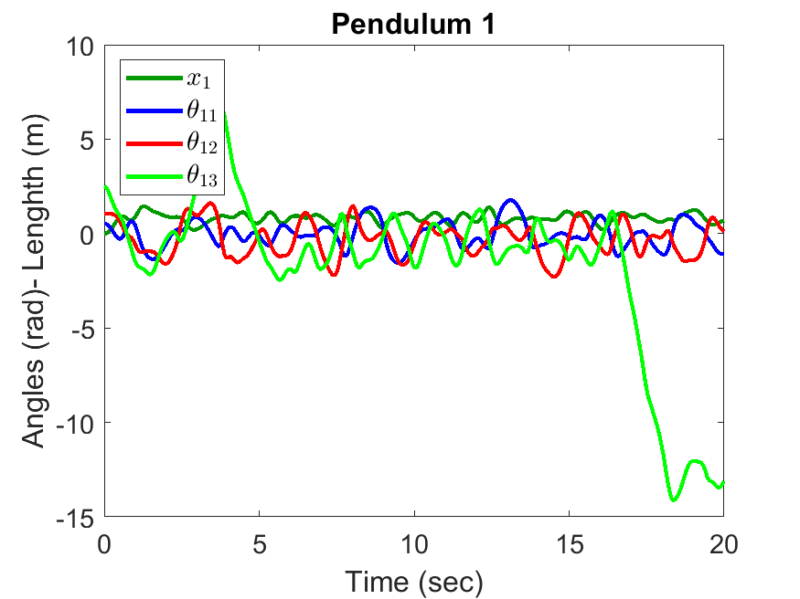
Triple Pendulum #1 Position and Anlges:
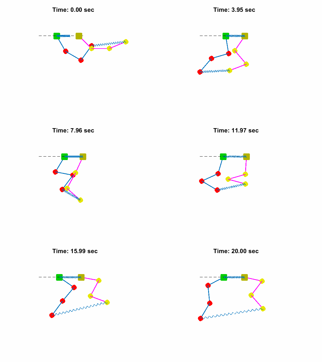
| Triple Pendulum #1 Position and Anlges: | Animated Response: |
|---|---|
|
|
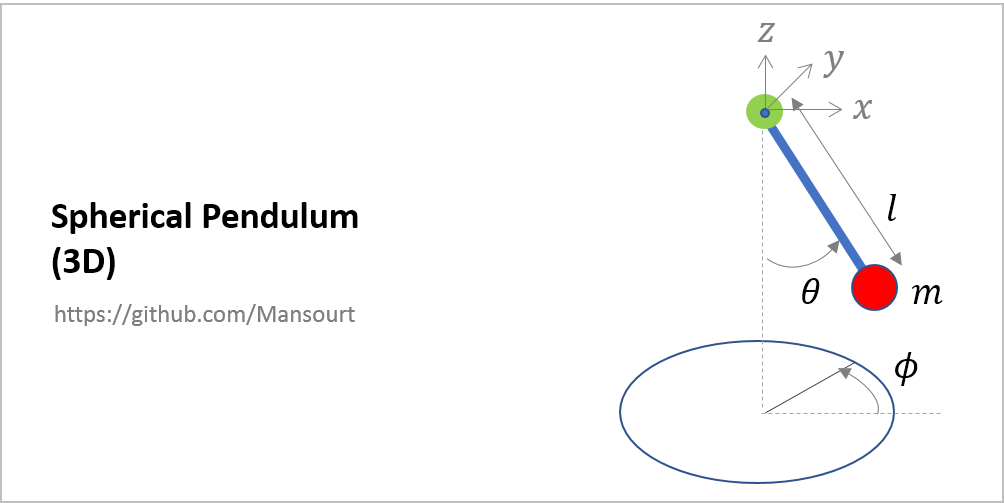
Problem Definition:
|
The simulation results are based on the following Values:
% List of Parameter Values
m0 = 1;
l0 = 2;
g0 = 9.81;

% Initial Conditions
th0  = 50;
phi0 = 0;
Dth0 = 0;
Dphi0 = 75;
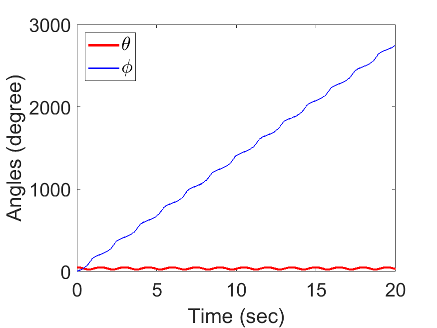
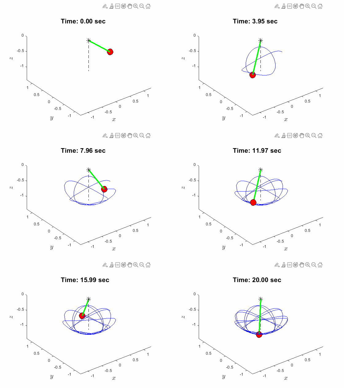
Spherical Pendulum Anlges:
| Spherical Pendulum Anlges: | Animated Response: |
|---|---|
|
|
Email: smtoraabi@ymail.com | mtmansourt@gmail.com
Citar como
mansour torabi (2026). Matlab Euler-Lagrange Library (https://github.com/Mansourt/Matlab_Euler-Lagrange_Library_for_Deriving_Equations_of_Dynamic_Systems/releases/tag/v1.5), GitHub. Recuperado .
Información general
- Versión 1.5 (10,5 MB)
-
Ver licencia en GitHub
Compatibilidad con la versión de MATLAB
- Compatible con cualquier versión
Compatibilidad con las plataformas
- Windows
- macOS
- Linux
| Versión | Publicado | Notas de la versión | Action |
|---|---|---|---|
| 1.5 | See release notes for this release on GitHub: https://github.com/Mansourt/Matlab_Euler-Lagrange_Library_for_Deriving_Equations_of_Dynamic_Systems/releases/tag/v1.5 |
||
| 1.4 | See release notes for this release on GitHub: https://github.com/Mansourt/Matlab_Euler-Lagrange_Library_for_Deriving_Equations_of_Dynamic_Systems/releases/tag/v1.4 |
||
| 1.3 | See release notes for this release on GitHub: https://github.com/Mansourt/Matlab_Euler-Lagrange_Library_for_Deriving_Equations_of_Dynamic_Systems/releases/tag/v1.3 |
||
| 1.2 | See release notes for this release on GitHub: https://github.com/Mansourt/Matlab_Euler-Lagrange_Library_for_Deriving_Equations_of_Dynamic_Systems/releases/tag/v1.2 |
||
| 1.1 | See release notes for this release on GitHub: https://github.com/Mansourt/Matlab_Euler-Lagrange_Library_for_Deriving_Equations_of_Dynamic_Systems/releases/tag/v1.1 |
||
| 1.0 |


