Generate Data for AI-Based 5G MIMO Channel Estimation

R2026b

Since R2026b

This example generates data to train a neural network for channel estimation in a 5G NR MIMO downlink. It uses a 5G PDSCH receiver to produce channel estimates at different SNR values and fading channel conditions. Use the data you generate in this example to build, train, and compare multiple neural network architectures in the Train and Evaluate Neural Networks for 5G MIMO Channel Estimation example.

The example covers the following stages:

• System and DM-RS Configuration: Configure the antenna setup, DM-RS pilot density, and resource grid structure used throughout the example.

• Slot Simulation: Simulate one slot through the transmitter, fading channel, and receiver chain up to channel estimation to produce a received resource grid, channel estimates at three tap points, and the OFDM channel response (referred to as perfect channel in the rest of the example).

• Neural Network Input Representations: Visualize and compare the three channel estimation representations used as neural network inputs (practical, LS-interp, LS-sparse), each offering a different tradeoff between noise suppression and bias.

• Generate Training Data: Repeat the slot simulation thousands of times with randomized channel conditions, then preprocess into neural-network-ready training arrays with feature-wise linear modulation (FiLM) conditioning inputs.

System and DM-RS Configuration

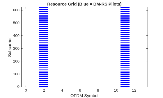
Configure a 5G NR downlink with 2x2 MIMO. The demodulation reference signal (DM-RS) configuration uses DMRSAdditionalPosition=1, placing pilots in 2 OFDM symbols per slot (indices 2 and 11), and ConfigType=1 provides 6 pilot subcarriers per RB, which results in approximately 7% resource element (RE) overhead. At moderate Doppler (up to approximately 100 Hz with TDL-C, 300 ns delay spread), 2 time-domain pilot symbols are sufficient for the practical estimator to reach 100% throughput at high SNR. At higher Doppler or longer delay spreads, the practical estimator degrades, leaving more room for neural networks to improve.

simParameters = hDeepLearningChanEstSimParameters();
disp("Carrier: " + simParameters.Carrier.NSizeGrid + " RBs, " ...
    + simParameters.Carrier.SubcarrierSpacing + " kHz SCS")

Carrier: 52 RBs, 15 kHz SCS

disp("Antenna: " + simParameters.NTxAnts + " Tx x " ...
    + simParameters.NRxAnts + " Rx, " ...
    + simParameters.PDSCH.NumLayers + " layers")

Antenna: 2 Tx x 2 Rx, 2 layers

disp("DM-RS: DMRSAdditionalPosition=" + simParameters.PDSCH.DMRS.DMRSAdditionalPosition ...
    + ", ConfigType=" + simParameters.PDSCH.DMRS.DMRSConfigurationType)

DM-RS: DMRSAdditionalPosition=1, ConfigType=1

disp("Modulation: " + string(simParameters.PDSCH.Modulation))

Modulation: 16QAM

DM-RS Pilot Structure

Visualize the resource grid for the first port to confirm the pilot placement. The blue pixels show DM-RS pilots. With DMRSAdditionalPosition=1, 2 of 14 OFDM symbols carry pilots (6 of 12 subcarriers per RB each).

carrier = simParameters.Carrier;
pdsch = simParameters.PDSCH;
dmrsIndices = nrPDSCHDMRSIndices(carrier, pdsch);
pdschIndices = nrPDSCHIndices(carrier, pdsch);
gridMap = nrResourceGrid(carrier);
gridMap(pdschIndices(:,1)) = 1;
gridMap(dmrsIndices(:,1)) = 2;
Nsc = size(gridMap,1);
Nsym = size(gridMap,2);

Throughout this example, $$N_{sc}$$, $$N_{sym}$$, and $$N_{coeff}$$ denote the number of subcarriers, OFDM symbols per slot, and channel coefficients ($$N_{Rx}$$*$$N_{Layers}$$), respectively.

figure
imagesc(0:Nsym-1, 0:Nsc-1, gridMap)
xlabel("OFDM Symbol")
ylabel("Subcarrier")
title("Resource Grid (Blue = DM-RS Pilots)")
axis xy
colormap([1 1 1; 0 0 1])

Slot Simulation

Simulate a single slot to illustrate the transmit, channel, and receive stages up to channel estimation. The example uses 20 dB SNR, 100 Hz Doppler, and a TDL-C channel with a delay spread of 300 ns. The Generate Training Data section repeats this simulation thousands of times with randomized SNR, Doppler, delay spread, and channel profile to build a training data set.

Configure Channel and Precoding

Configure a TDL-C fading channel. In a MIMO system, the gNodeB applies precoding to focus energy along the dominant spatial directions. Here, SVD precoding weights are computed per precoding resource block group (PRG) from an initial channel estimate. With SVD precoding, the effective channel has orthogonal columns across layers, so each element of the effective channel matrix (one per receive antenna per layer) is independent. The neural network operates on one antenna-layer pair at a time rather than the full MIMO signal, which lets a single network handle any antenna configuration. Each antenna-layer pair becomes one training sample for the neural network.

channel = nrTDLChannel;
channel.DelayProfile = "TDL-C";
channel.DelaySpread = 300e-9;
channel.MaximumDopplerShift = 100;
channel.NumTransmitAntennas = simParameters.NTxAnts;
channel.NumReceiveAntennas = simParameters.NRxAnts;
channel.ChannelResponseOutput = "ofdm-response";
waveformInfo = nrOFDMInfo(carrier);
channel.SampleRate = waveformInfo.SampleRate;

Get an initial channel estimate and compute SVD precoding weights per PRG. The precoder is constant within each PRG, so the effective channel $$H_{eff}=H\cdot W$$ is also approximately constant across those subcarriers. This property makes each PRG a natural tile boundary for the neural network input. The network processes the resource grid in PRG-sized chunks ($$PRGSizeRBs\times 12$$ subcarriers $$\times$$ 14 symbols $$\times$$ $$N_{coeff}$$ coefficients), making it scalable to any bandwidth composed of multiple PRGs.

simParameters.PRGSizeRBs = 4; % 48 subcarriers
estGrid = hGetInitialChannelEstimate(channel, carrier);
W = hSVDPrecoders(carrier, pdsch, estGrid, simParameters.PRGSizeRBs);

Build Resource Grid

Precode both PDSCH data symbols and DM-RS pilots with the same weights. The UE does not know the precoder. It estimates the effective (precoded) channel $$H_{eff}=H\cdot W$$ directly from the precoded pilots.

txGrid = nrResourceGrid(carrier, simParameters.NTxAnts);
[pdschInd, pdschInfo] = nrPDSCHIndices(carrier, pdsch);
cws = randi([0 1], pdschInfo.G, 1);
pdschSym = nrPDSCH(carrier, pdsch, cws);
[antSym, antInd] = nrPDSCHPrecode(carrier, pdschSym, pdschInd, W);
txGrid(antInd) = antSym;

Generate DM-RS indices and symbols. For ConfigType=1, pilots occupy every second subcarrier within a DM-RS symbol (Comb-2).

dmrsInd = nrPDSCHDMRSIndices(carrier, pdsch);
dmrsSym = nrPDSCHDMRS(carrier, pdsch);
cdmLen = pdsch.DMRS.CDMLengths;
[antSym, antInd] = nrPDSCHPrecode(carrier, dmrsSym, dmrsInd, W);
txGrid(antInd) = antSym;

Transmit, Add Noise, and Demodulate

Pass the signal through the fading channel, add AWGN at 20 dB per-RE per receive antenna SNR, and OFDM-demodulate.

txWaveform = nrOFDMModulate(carrier, txGrid);
chInfo = info(channel);
txWaveform = [txWaveform; zeros(chInfo.MaximumChannelDelay, size(txWaveform,2))];
[rxWaveform, ofdmResponse, offset] = channel(txWaveform, carrier);

% Perfect channel (ground truth after precoding)
perfectChan = hPrecodeChannelEstimate(carrier, ofdmResponse, permute(W,[2 1 3]));

% Add noise at 20 dB SNR
SNRdB = 20;
Nfft = waveformInfo.Nfft;
NRxAnts = simParameters.NRxAnts;
SNR = 10^(SNRdB/10);
N0 = 1/sqrt(NRxAnts*Nfft*SNR);
noise = N0*randn(size(rxWaveform),"like",rxWaveform);
rxWaveform = rxWaveform + noise;
% To align to the start of the OFDM symbol, remove channel delay offset
rxWaveform = rxWaveform(1+offset:end, :);

% OFDM demodulate
rxGrid = nrOFDMDemodulate(carrier, rxWaveform);

Channel Estimation

Channel estimation uses the DM-RS pilot symbols. The receiver computes a least squares (LS) estimate by dividing received symbols by known pilot values, yielding noisy channel estimates at pilot subcarrier positions. CDM despreading then separates co-multiplexed antenna ports by averaging within each CDM group. Further processing reduces estimation noise and produces channel estimates at all RE positions.

As shown in this diagram, the nrChannelEstimate function implements LS and CDM despreading, then applies three additional processing stages.

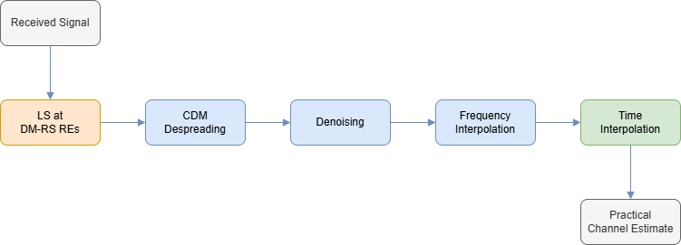
1. Denoising: IFFT, raised-cosine windowing within the cyclic prefix length, FFT. An SNR-adaptive moving average further smooths the pilot estimates.

2. Frequency interpolation: Spline from pilot subcarriers to all subcarriers.

3. Time interpolation: Linear interpolation between DM-RS symbols to fill non-pilot OFDM symbols.

The result is a full-grid channel estimate with effective noise suppression. This example refers to it as the practical estimate.

[hPractical, noiseEst] = nrChannelEstimate(carrier, rxGrid, dmrsInd, dmrsSym, ...
    CDMLengths=cdmLen, PRGBundleSize=simParameters.PRGSizeRBs);

Alternative Inputs for Neural Network Training

Each estimation stage adds noise suppression but also introduces bias. The estimate systematically deviates from the true channel where the smoothing assumptions break down. LS at pilot positions is unbiased but noisy. Linear interpolation fills the grid but cannot track nonlinear channel variations between pilots. The practical estimator (nrChannelEstimate) adds denoising and averaging, which works well at low-to-moderate SNR. However, it creates a performance floor at high SNR and high Doppler, where the channel changes faster than the interpolation can follow.

A neural network can learn to denoise and interpolate without these fixed assumptions. The choice of input representation determines what the network must learn. Give it the practical estimate and it refines an already good starting point; give it raw LS at the DM-RS REs only and it must reconstruct the entire grid from scratch. As shown in this diagram, two simpler representations skip the denoising and averaging stages.

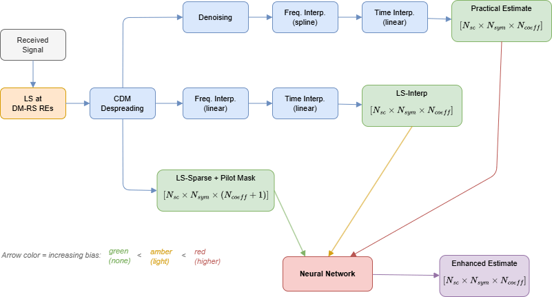
LS-Interp: This representation applies CDM despreading followed by linear interpolation in frequency and time. It does not apply denoising or averaging, so noise on pilot observations propagates directly to the full-grid estimate. Linear interpolation also introduces bias at positions where the channel does not vary linearly between pilots.

hLSInterp = hLSChannelEstimate(rxGrid,dmrsInd,dmrsSym,CDMLengths=cdmLen,PRGSizeRBs=simParameters.PRGSizeRBs);

LS-Sparse: This representation contains LS values only at pilot REs after CDM despreading and zeros elsewhere. The network must reconstruct the full time-frequency grid from minimal observations. A binary pilot mask indicates valid positions and is concatenated as an extra channel in the network input ($$N_{coeff}+1$$).

[~, ~, rawEst] = hLSChannelEstimate(rxGrid, dmrsInd, dmrsSym, CDMLengths=cdmLen, Interpolation=false);
hLSSparse = rawEst.PilotEstimates;
pilotREMask = rawEst.PilotMask;

Neural Network Input Representations

Visualize the first PRG (48 subcarriers x 14 symbols) for each representation alongside the perfect channel.

prgIdx = 1:48;   % valid only if carrier.NStartGrid = 0
plotInputRepresentation(hLSSparse,hLSInterp,hPractical,perfectChan,prgIdx);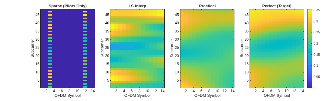

Generate Training Data

Generate a data set of channel realizations by running the slot simulation thousands of times with randomized channel conditions. The hGenerate5GChannelEstimationData helper returns all three representations (practical, LS-interp, LS-sparse) and the perfect channel for each realization. The hPrepareChannelEstimationTrainingData helper function then preprocesses the raw data into training and validation arrays ready for neural network training.

Set Channel and Training Parameters

Define the channel and training distribution. The training range covers Doppler from 5 to 400 Hz (pedestrian to vehicular at 3.5 GHz), delay spread from 30 to 1000 ns (indoor to urban macro), and three delay profiles (TDL-A, TDL-C, TDL-D) spanning NLOS and LOS conditions. SNR ranges from –5 to 25 dB. During generation, each parameter is drawn uniformly from its specified range, and the delay profile is selected randomly from the specified set. For faster interactive execution, set the numRealizations variable to 256 . For more accurate training, use 4096.

dopplerRange = [5 400];
delaySpreadRange = [30 1000];
delayProfiles = {"TDL-A", "TDL-C", "TDL-D"}; % 2 NLOS + 1 LOS
snrRange = [-5 25];
numRealizations = 256;

Generate Channel Realizations

The hGenerate5GChannelEstimationData helper function performs the same simulation (channel, precoding, noise, multi-tap estimation) but in a parfor loop over many realizations with randomized SNR, Doppler, delay spread, and profile. One call returns matched representations for all realizations.

rawData = hGenerate5GChannelEstimationData(numRealizations, ...
    SNRRange=snrRange, DopplerRange=dopplerRange, ...
    DelaySpreadRange=delaySpreadRange, ...
    DelayProfiles=delayProfiles, ...
    SimParameters=simParameters, ...
    PrintProgress=true);
disp("Realizations: " + size(rawData.perfect, 4))

Realizations: 256

disp("Grid size: " + rawData.Nsc + " SC x " + rawData.Nsym + " symbols x " ...
    + rawData.nSpatial + " spatial dimensions (nRx x nLayers)")

Grid size: 624 SC x 14 symbols x 4 spatial dimensions (nRx x nLayers)

Preprocess Training Data

The raw channel data is complex-valued and spans the full carrier bandwidth. Several preprocessing steps adapt it for efficient neural network training:

• Reduce input size: The full bandwidth grid is tiled into PRG-sized sub-grids (4 RBs = 48 subcarriers), reducing network complexity from thousands of subcarriers to a fixed 48.

• Enable bandwidth generalization: Because the precoder is constant within each PRG, the tile boundaries align with a known structural property of the system. The network processes one tile at a time and generalizes to any carrier bandwidth.

• Antenna-layer processing: With SVD precoding, the effective channel has orthogonal columns across layers. Each element of the effective channel matrix (one per receive antenna per layer) is independent and is treated as a separate training sample, making the network agnostic to antenna configuration.

• Normalization: Per-sample RMS normalization removes absolute power level, letting the network focus on channel shape rather than magnitude.

• Side information: The estimated SNR is provided to the network as a scalar conditioning input via FiLM layers. By telling the network the current SNR, a single set of weights can adapt its denoising and interpolation strength to the operating point rather than requiring separate models for each SNR regime.

All three input representations follow the same five-step pipeline:

1. Train/validation split

2. Antenna-layer processing and real/imaginary split

3. PRG tiling

4. Per-sample RMS normalization

5. Side information (SNR conditioning)

The following subsection describes each step using the practical representation as an example. The hPrepareChannelEstimationTrainingData helper function performs these steps in one call. Use this helper function to generate data for all three input representations.

Preprocessing Pipeline

The raw data has shape $$[N_{sc}\times N_{sym}\times N_{coeff}\times N]$$, where $$N_{sc}$$ is the number of subcarriers, $$N_{sym}$$ is the number of OFDM symbols per slot, $$N_{coeff}=N_{Rx}\times N_{Layers}$$ is the number of effective channel coefficients, and $$N$$ is the number of realizations.

1. Train/validation split. Split by realization index, not by PRG. PRGs from the same realization share the same channel statistics (delay profile, Doppler, SNR), so placing some in training and others in validation overestimates generalization performance.

[Nsc, Nsym, Ncoeff, N] = size(rawData.practical);
perm = randperm(RandStream("twister",Seed=42),N);
nVal = round(N * 0.1);
valIdx = perm(1:nVal);
trainIdx = perm(nVal+1:end);

2. Antenna-layer processing and real/imaginary split. With SVD precoding, the effective channel has orthogonal columns across layers, so the $$N_{coeff}$$ antenna-layer pairs (one per receive antenna per layer) are approximately independent. Each pair is treated as a separate sample with 2 real channels (real and imaginary parts). Processing antenna-layer pairs independently makes the network agnostic to the antenna configuration. A network trained on 2x2 generalizes to 4x4 without retraining. The data set grows by a factor of $$N_{coeff}$$.

nCh = 2;
Ntotal = N * Ncoeff;
inputRI = zeros(Nsc, Nsym, nCh, Ntotal, 'single');
for k = 1:Ncoeff
    idx = (k-1)*N + (1:N);
    inputRI(:,:,1,idx) = real(rawData.practical(:,:,k,:));
    inputRI(:,:,2,idx) = imag(rawData.practical(:,:,k,:));
end

3. PRG tiling. Tile the full bandwidth into non-overlapping 4-RB (48 subcarrier) sub-grids. Each [624 x 14 x 2] grid becomes 13 independent training samples of [48 x 14 x 2]. At inference, the same tiling makes the network applicable to any bandwidth.

prgSC = PRGSizeRBs * 12;       % 48
numPRGs = floor(Nsc / prgSC);  % 13
trainX = zeros(prgSC, Nsym, nCh, numPRGs*nTrain, 'single');
for n = 1:nTrain
    for p = 1:numPRGs
        sc0 = (p-1)*prgSC + 1;
        trainX(:,:,:,idx) = inputRI(sc0:sc0+prgSC-1, :, :, trainIdxAll(n));
    end
end

4. Per-sample RMS normalization. Normalize each sample by its RMS amplitude, applying the same scale to both input and label. The network learns channel shape, not absolute power level.

sampleRMS = rms(trainX, [1 2 3]);
trainX = trainX ./ sampleRMS;
trainT = trainT ./ sampleRMS;

5. Side information (SNR conditioning). The estimated SNR is provided to the network as a scalar conditioning input for FiLM layers, enabling a single network to adapt its denoising strength to the current operating point. SNR is normalized to the range 0 to 1 over the training range:

trainSNR = (snrEstimate(trainIdx) - snrRange(1)) / diff(snrRange);

Prepare Training Representations

Call hPrepareChannelEstimationTrainingData for each input representation. The helper function performs the five-step pipeline and returns a structure with training/validation arrays and conditioning inputs.

Practical: This representation uses the full-grid estimate from nrChannelEstimate (denoised + interpolated).

pracData = hPrepareChannelEstimationTrainingData(rawData.practical, rawData.perfect, ...
    rawData.snrEstPractical, PRGSizeRBs=simParameters.PRGSizeRBs, SNRRange=snrRange);
disp("Practical training samples: " + size(pracData.trainX,4) + " [" + ...
    size(pracData.trainX,1) + "x" + size(pracData.trainX,2) + "x" + ...
    size(pracData.trainX,3) + "]")

Practical training samples: 11960 [48x14x2]

LS-Interp: This representation uses the linearly interpolated full-grid estimate, same shape as practical, but no denoising or averaging.

interpData = hPrepareChannelEstimationTrainingData(rawData.lsInterp, rawData.perfect, ...
    rawData.snrEstInterp, PRGSizeRBs=simParameters.PRGSizeRBs, SNRRange=snrRange);
disp("LS-Interp training samples: " + size(interpData.trainX,4) + " [" + ...
    size(interpData.trainX,1) + "x" + size(interpData.trainX,2) + "x" + ...
    size(interpData.trainX,3) + "]")

LS-Interp training samples: 11960 [48x14x2]

LS-Sparse: This representation uses the raw LS estimates at pilot positions only, with a binary mask indicating valid REs. RMS normalization uses only pilot positions (non-pilot values are zero).

sparseData = hPrepareChannelEstimationTrainingData(rawData.lsSparse, rawData.perfect, ...
    rawData.snrEstSparse, PRGSizeRBs=simParameters.PRGSizeRBs, SNRRange=snrRange, ...
    MaskChannel=rawData.pilotMask);
disp("LS-Sparse: " + size(sparseData.trainX, 3) + " signal channels + " + ...
    "mask [" + size(sparseData.trainMask,1) + "x" + ...
    size(sparseData.trainMask,2) + "x" + size(sparseData.trainMask,3) + "]")

LS-Sparse: 2 signal channels + mask [48x14x1]

Save Training Data

Save the three preprocessed representations and the generation parameters. To reuse this data in a future session, load the file before running the training example. The training example skips data generation if the variables already exist in memory.

trainingParams.dopplerRange = dopplerRange;
trainingParams.delaySpreadRange = delaySpreadRange;
trainingParams.delayProfiles = delayProfiles;
trainingParams.snrRange = snrRange;

filename = "chanEstTrainingData_" + string(datetime("now", Format="yyyyMMdd_HHmmss")) + ".mat";
save(filename, ...
    "pracData", "interpData", "sparseData", ...
    "trainingParams", "simParameters");
fprintf("Saved training data to %s (%.1f MB)\n", filename, dir(filename).bytes/1e6)

Saved training data to chanEstTrainingData_20260817_162013.mat (253.6 MB)

Further Exploration

To build, train, and compare multiple architectures (Vision Transformer, CENet, ResDenoiser) using this data, see the Train and Evaluate Neural Networks for 5G MIMO Channel Estimation example. You can also try these explorations:

• Mixed-SCS training: Loop over [15, 30, 60, 120] kHz, generating data at each SCS with hDeepLearningChanEstSimParameters(SubcarrierSpacing=scs). The pilot mask and grid dimensions are identical across SCS values, so results concatenate directly along the realization dimension. Add frequency selectivity FiLM conditioning (freqVar) to make the network SCS aware.

• Extend delay profiles: Add TDL-B and TDL-E to cover all 3GPP profiles. The network generalizes via training data diversity.

• Increase bandwidth: Change NSizeGrid to 106 or 273 RBs. The PRG tiling makes the networks bandwidth agnostic.

• MIMO scaling: Generate 4x4 or 8x2 antenna configurations to verify that antenna-layer processing generalizes across array sizes.

• Visualize parameter distributions: Plot histograms of estimated vs. true SNR to understand conditioning input accuracy across the training range.

• Compare representations: Compute NMSE of each input representation against the perfect channel (before any NN) to quantify the starting-point quality gap.

Helper Functions

function plotInputRepresentation(hLSSparse,hLSInterp,hPractical,perfectChan,prgIdx)
fig = figure;
fig.Position(3) = fig.Position(3) * 2;
tiledlayout(1,4)
vals = [abs(hLSSparse(prgIdx,:,1,1)); abs(hLSInterp(prgIdx,:,1,1)); ...
    abs(hPractical(prgIdx,:,1,1)); abs(perfectChan(prgIdx,:,1,1))];
colorLimits = [min(vals(:)), max(vals(:))];
nexttile
imagesc(abs(hLSSparse(prgIdx,:,1,1))); 
axis xy
clim(colorLimits)
title("Sparse (Pilots Only)"); 
xlabel("OFDM Symbol"); 
ylabel("Subcarrier")
nexttile
imagesc(abs(hLSInterp(prgIdx,:,1,1))); 
axis xy
clim(colorLimits)
title("LS-Interp"); 
xlabel("OFDM Symbol"); 
ylabel("Subcarrier")
nexttile
imagesc(abs(hPractical(prgIdx,:,1,1))); 
axis xy
clim(colorLimits)
title("Practical"); 
xlabel("OFDM Symbol"); 
ylabel("Subcarrier")
nexttile
imagesc(abs(perfectChan(prgIdx,:,1,1))); 
axis xy
clim(colorLimits)
title("Perfect (Target)"); 
xlabel("OFDM Symbol"); 
ylabel("Subcarrier")
colorbar
end