FMCW Patch Antenna Array

Design Parameters

Set up the center frequency and the frequency band. The velocity of light is assumed to be that of vacuum.

fc = 77e9;
fmin = 73e9;
fmax = 80e9;
vp = physconst("lightspeed");
lambda = vp/fc;

Create 2-by-4 Array

Hypothetical Element Pattern

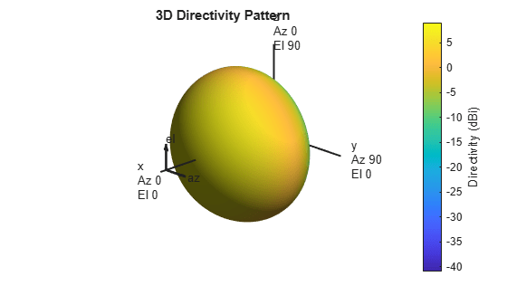
The FMCW antenna array is intended for a forward radar system designed to look for and prevent a collision. Therefore, begin with a hypothetical antenna element that has the significant pattern coverage in one hemisphere. A cosine antenna element would be an appropriate choice.

cosineElement = phased.CosineAntennaElement;
cosineElement.FrequencyRange = [fmin fmax];
cosinePattern = figure;
pattern(cosineElement,fc)

Ideal Array Pattern

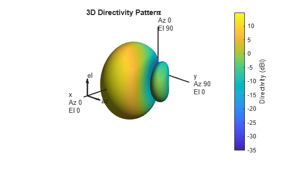
The array itself needs to be mounted on or around the front bumper. The array configuration we investigate is similar to that mentioned in [1], i.e. a 2-by-4 rectangular array.

Nrow = 2;
Ncol = 4;
fmcwCosineArray = phased.URA;
fmcwCosineArray.Element = cosineElement;
fmcwCosineArray.Size = [Nrow Ncol];
fmcwCosineArray.ElementSpacing = [0.5*lambda 0.5*lambda];
cosineArrayPattern = figure;
pattern(fmcwCosineArray,fc);

Design Realistic Patch Antenna

The Antenna Toolbox™ has several antenna elements that could provide hemispherical coverage. Choose the patch antenna element and design it at the frequency of interest. The patch length is approximately half-wavelength at 77 GHz and the width is 1.5 times the length, for improving the bandwidth.

patchElement = design(patchMicrostrip,fc);

Since the default patch antenna geometry in the Antenna Toolbox library has its maximum radiation directed towards zenith, rotate the patch antenna by 90 degrees about the y-axis so that the maximum would now occur along the x-axis. This is also the boresight direction for arrays in Phased Array System Toolbox™.

patchElement.Tilt = 90;
patchElement.TiltAxis = [0 1 0];
figure
show(patchElement)
axis tight
view(140,20)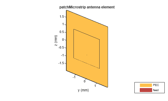

Isolated Patch Antenna 3D Pattern and Resonance

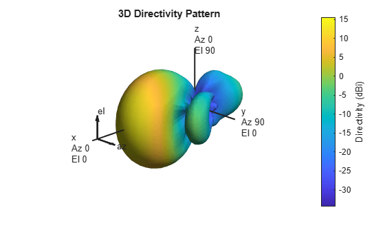
3D Directivity Pattern

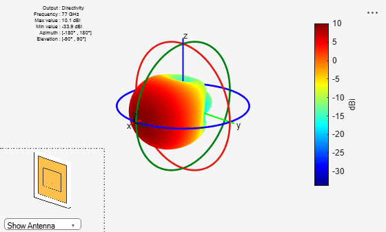
Plot the pattern of the patch antenna at 77 GHz. The patch is a medium gain antenna with the peak directivity around 6 - 9 dBi.

pattern(patchElement,fc)

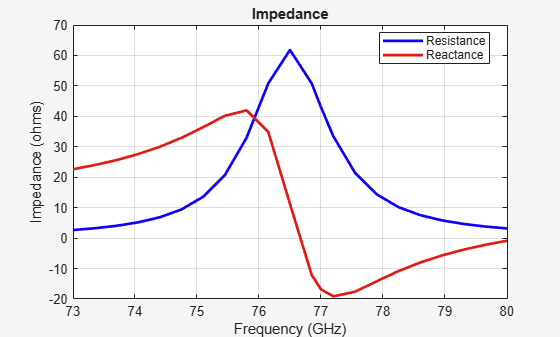
Resonance

The patch is radiating in the correct mode with a pattern maximum at azimuth = elevation = 0 degrees. Since the initial dimensions are an approximation, check the input impedance behavior.

Numfreqs = 21;
freqsweep = unique([linspace(fmin,fmax,Numfreqs) fc]);
impedance(patchElement,freqsweep);

Establish Bandwidth

Plot the reflection coefficient of the patch to confirm a good impedance match. It is typical to consider the value $$S_{11}=-10dB$$ as a threshold value for determining the antenna bandwidth.

s = sparameters(patchElement,freqsweep);
figure
rfplot(s,'m-.')
hold on
line(freqsweep/1e09,ones(1,numel(freqsweep))*-10,LineWidth=1.5)
hold off

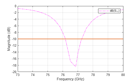
The deep minimum at 77 GHz indicates a good match to 50. The antenna bandwidth is slightly greater than 1 GHz. Thus, the frequency band is from 76.5 GHz to 77.5 GHz.

Confirm Pattern at Center and Corner Frequencies

Confirm that the pattern at the corner frequencies of the band remains nearly the same. The pattern plots at 76.5 GHz and 77.5 GHz are shown below.

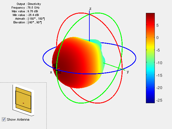
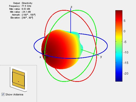
It is a good practice to check pattern behavior over the frequency band of interest in general.

Create Array from Isolated Radiators and Plot Pattern

Create the uniform rectangular array (URA), but this time use the isolated patch antenna as the individual element. We choose spacing $$\lambda /2$$ at the upper frequency of the band i.e. 77.6 GHz.

fc2 = 77.6e9;
lambda_fc2 = vp/77.6e9;
fmcwPatchArray = phased.URA;
fmcwPatchArray.Element = patchElement;
fmcwPatchArray.Size = [Nrow Ncol];
fmcwPatchArray.ElementSpacing = [0.5*lambda_fc2 0.5*lambda_fc2];

Plot the pattern for the patch antenna array so constructed. Specify a 5 degree separation in azimuth and elevation to plot the 3D pattern.

az = -180:5:180;
el = -90:5:90;
patchArrayPattern = figure;
pattern(fmcwPatchArray,fc,az,el);

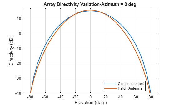
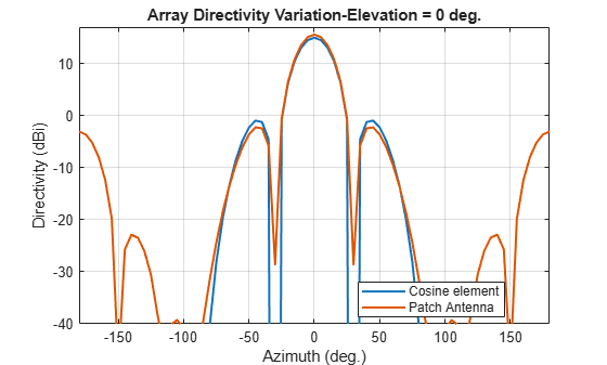
Plot Pattern Variation in Two Orthogonal Planes

Compare the pattern variation in 2 orthogonal planes for the patch antenna array and the cosine element array. Both arrays ignore mutual coupling.

[Dcosine_az_zero,~,eln] = pattern(fmcwCosineArray,fc,0,el);
[Dcosine_el_zero,azn] = pattern(fmcwCosineArray,fc,az,0);
[Dpatch_az_zero,~,elp] = pattern(fmcwPatchArray,fc,0,el);
[Dpatch_el_zero,azp] = pattern(fmcwPatchArray,fc,az,0);

elPattern = figure;
plot(eln,Dcosine_az_zero,eln,Dpatch_az_zero,LineWidth=1.5)
axis([min(eln) max(eln) -40 17])
grid on
xlabel("Elevation (deg.)")
ylabel("Directivity (dBi)")
title("Array Directivity Variation-Azimuth = 0 deg.")
legend("Cosine element","Patch Antenna",Location="best")

azPattern = figure;
plot(azn,Dcosine_el_zero,azn,Dpatch_el_zero,LineWidth=1.5)
axis([min(azn) max(azn) -40 17])
grid on
xlabel("Azimuth (deg.)")
ylabel("Directivity (dBi)")
title("Array Directivity Variation-Elevation = 0 deg.")
legend("Cosine element","Patch Antenna",Location="best")

Discussion

The cosine element array and the array constructed from isolated patch antennas, both without mutual coupling, have similar pattern behavior around the main beam in the elevation plane (azimuth = 0 deg). The patch-element array has a significant back lobe as compared to the cosine-element array. Using the isolated patch element is a useful first step in understanding the effect that a realistic antenna element would have on the array pattern. However, in the realistic array analysis, mutual coupling must be considered. Since this is a small array (8 elements in 2-by-4 configuration), the individual element patterns in the array environment could be distorted significantly. As a result, it is not possible to replace the isolated element pattern with an embedded element pattern. A full-wave analysis must be performed to understand the effect of mutual coupling on the overall array performance.

Reference

[1] Kulke, R., S. Holzwarth, J. Kassner, A. Lauer, M. Rittweger, P. Uhlig and P. Weigand. “24 GHz Radar Sensor integrates Patch Antenna and Frontend Module in single Multilayer LTCC Substrate.” (2005).