Main Content

chromosomeplot

Plot chromosome ideogram with G-banding pattern

Description

chromosomeplot(CytoData) plots the ideogram of all chromosomes, using information from cytogenetic G-banding data CytoData.

example

chromosomeplot(CytoData,ChromNum) plots the ideogram of a single chromosome specified by ChromNum.

example

chromosomeplot(___,Name=Value) specifies additional options using one or more name-value arguments.

example

Examples

collapse all

Read the cytogenetic banding information for Homo sapiens into a structure.

hs_cytobands = cytobandread('hs_cytoBand.txt')
hs_cytobands = struct with fields:
     ChromLabels: {862×1 cell}
    BandStartBPs: [862×1 int32]
      BandEndBPs: [862×1 int32]
      BandLabels: {862×1 cell}
       GieStains: {862×1 cell}

Plot the entire chromosome ideogram.

chromosomeplot(hs_cytobands);
title('Human Karyogram')

Figure contains an axes object. The hidden axes object with title Human Karyogram contains 1088 objects of type patch, line, text.

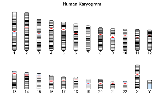
You can display the ideogram of a specific chromosome by right-clicking it in the plot, then selecting Display in New Figure > Vertical or Horizontal.

You can also programmatically display the ideogram of a specific chromosome, set the orientation, and the units used in the data tip to kilo base pairs.

chromosomeplot(hs_cytobands, 15, 'Orientation', 2, 'Unit', 2);

Figure contains an axes object. The hidden axes object contains 107 objects of type patch, line, text.

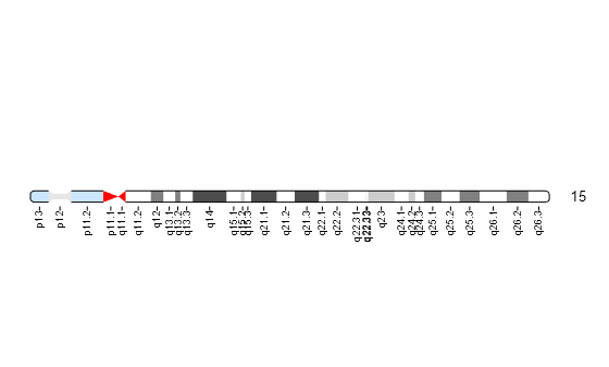
Hover over the chromosome to view a data tip. To get more information about a specific band, select the Data Cursor button on the toolbar and click the band in the plot. Use the context menu (right-click) to see more options such as deleting or creating a data tip.

Load the array-based CGH (aCGH) data from the Coriell cell line study (Snijders, A. et al., 2001).

load coriell_baccgh

Use the cghcbs function to analyze chromosome 10 of sample 3 (GM05296) of the aCGH data and return copy number variance (CNV) data in a structure, S. Plot the segment means over the original data for only chromosome 10 of sample 3.

S = cghcbs(coriell_data,'sampleindex',3,'chromosome',10,...
           'showplot',10);
Analyzing: GM05296. Current chromosome 10

Figure contains an axes object. The axes object with title GM05296 - Chr 10, xlabel Genomic Position, ylabel Log2(Ratio) contains 4 objects of type line. One or more of the lines displays its values using only markers

Use the chromosomeplot function with the 'addtoplot' option to add the ideogram of chromosome 10 for Homo sapiens to the plot. Because the plot of the CNV data from the Coriell cell line study is in kb units, use the 'Unit' property to convert the ideogram data to kb units.

set(gcf,'color','w'); % Set the background of the figure to white.
chromosomeplot('hs_cytoBand.txt', 10, 'addtoplot', gca,...
               'Unit', 2);

Figure contains 2 axes objects. Axes object 1 with title GM05296 - Chr 10, xlabel Genomic Position, ylabel Log2(Ratio) contains 4 objects of type line. One or more of the lines displays its values using only markers Hidden axes object 2 contains 134 objects of type patch, line, text.

Input Arguments

collapse all

Cytogenetic G-banding data in bp units, specified as a structure, or character vector or string scalar representing the name of a file.

If CytoData is a structure, it must contain the cytogenetic G-banding data with the following fields:

  • ChromLabels

  • BandStartBPs

  • BandEndBPs

  • BandLabels

  • GieStains

The cytobandread function creates such a structure.

If CytoData is a file name, the file must contain cytogenetic G-banding data. For example, the file can be an NCBI ideogram text file or a UCSC Genome Browser cytoband text file.

The G bands distinguish different areas of the chromosome. For example, for the Homo sapiens ideogram, possible G bands are:

  • gneg — white

  • gpos25 — light gray

  • gpos50 — medium gray

  • gpos75 — dark gray

  • gpos100 — black

  • acen — red (centromere)

  • stalk — indented region (region with repeats)

  • gvar — light blue

Darker bands are AT-rich, while lighter bands are GC-rich.

Data Types: char | string | struct

Chromosome to plot, specified as a nonnegative scalar, "X", or "Y".

By default, the function plots ideograms for all chromosomes.

Data Types: double | char | string

Name-Value Arguments

collapse all

Specify optional pairs of arguments as Name1=Value1,...,NameN=ValueN, where Name is the argument name and Value is the corresponding value. Name-value arguments must appear after other arguments, but the order of the pairs does not matter.

Example: chromosomeplot(hs_cytobands,15,Orientation=2) plots chromosome 15 in the horizontal orientation.

Orientation of a specified chromosome to plot, specified as "Vertical" or 1 or "Horizontal" or 2.

You must specify a single chromosome for this name-value argument to work.

When plotting the ideogram of all chromosomes, the orientation is always vertical.

Data Types: double | char | string

Flag to display band labels of a specified chromosome, specified as a numeric or logical true (1) or false (0).

You must specify a single chromosome for this name-value argument to work.

Data Types: double | logical

Axes handle of a figure to which to add a single chromosome ideogram, specified as an axes handle.

If you use this property to add the ideogram to a plot of genomic data that is in units other than bp, use the Unit argument to convert the ideogram data to the appropriate units.

Tip

Before printing a figure containing an added chromosome ideogram, change the background to white by issuing the following command: set(gcf,'color','w').

Unit for the starting and ending genomic positions, specified as 1 (bp), 2 (kb), or 3 (mb).

This unit is used in the data tip displayed when you hover the cursor over chromosomes in the ideogram. This unit can also be used when using the AddToPlot argument to add the ideogram to a plot that is in units other than bp.

Data Types: double

Option to control the display of copy number variance data aligned to the chromosome ideogram, specified as a scalar structure.

Gains are shown in green to the right or above the ideogram, while losses are shown in red to the left or below the ideogram.

The structure has the following fields. Each field must contain the same number of elements.

FieldDescription
Chromosome

Either of the following:

  • Numeric vector containing the chromosome number on which each CNV is located.

    Note

    For the sex chromosome, X, use N, where N = number of autosomes + 1. For the sex chromosome, Y, use M, where M = number of autosomes + 2. For example, for Homo sapiens use 23 for X and 24 for Y, and for Mus musculus (lab mouse), use 20 for X and 21 for Y.

  • Character array containing the chromosome number on which each CNV is located.

    Note

    Using a character array lets you use the characters X and Y (instead of numbers) for sex chromosomes. However, all elements in the array must be the same width, which may require you to add spaces to some character vectors. For example:

    [' 1'; ' 2'; '10'; ' X']

    Or you can use the char function with a cell array to create a character array of the chromosome numbers and letters. For example:

    char({'1', '2', '10', 'X'})

CNVType

Numeric vector containing the type of each CNV, either 1 (loss) or 2 (gain).

Start

Numeric vector containing the starting genomic position of each CNV. Units must be in base pairs.

End

Numeric vector containing the ending genomic position of each CNV. Units must be in base pairs.

Data Types: struct

Version History

Introduced in R2007b