Online Training and Testing of PyTorch Model for CSI Feedback Compression

Since R2025a

This example shows how to perform online training and testing of a PyTorch® autoencoder-based neural network for channel state information (CSI) feedback compression.

In this example, you:

1. Train the autoencoder-based neural network using online training.

2. Test the trained neural network.

3. Compare the performance metrics of the complex input lightweight neural network (CLNet) PyTorch model across multiple compression factors.

Introduction

In 5G networks, efficient handling of CSI is crucial for optimizing downlink data transmission. Traditional methods rely on feedback mechanisms where the user equipment (UE) processes the channel estimate to reduce the CSI feedback data sent to the access node (gNB). However, an innovative approach involves using an autoencoder-based neural networks to compress and decompress the CSI feedback more effectively.

In this example, you define, train, test, and compare the performance of the following autoencoder model:

• Complex input lightweight neural network (CLNet): CLNet is a lightweight neural network designed for massive multiple-input multiple-output (MIMO) CSI feedback, which utilizes complex-valued inputs and attention mechanisms to improve accuracy while reducing computational overhead [1].

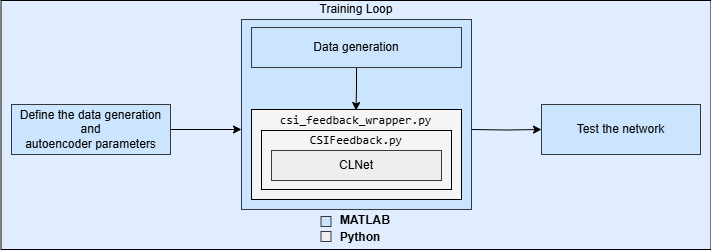
In deep learning, online training updates a model incrementally as new data arrives, while offline training model uses the entire data set at once. The diagram below shows online training for an autoencoder-based neural network using MATLAB® and Python® co-execution.

Set Up Python Environment

Set up the Python® environment as described in PyTorch Coexecution before running the example. Specify the full path of the Python executable to use below. The helperSetupPyenv function sets the Python Environment in MATLAB® based on the selected options and checks that the libraries listed in the requirements_csi_feedback.txt file are installed.

If you use Windows®, provide the path to the pythonw.exe file.

if ispc
    exePath = "..\python\pythonw.exe";
else    
    exePath = "../python/python/bin/python3";
end
exeMode = "OutOfProcess";
currentPenv = helperSetupPyenv(exePath,exeMode,'requirements_csi_feedback.txt');

Setting up Python environment
Parsing requirements_csi_feedback.txt 
Checking required package 'numpy'
Checking required package 'torch'
Required Python libraries are installed.

Specify Data Set Parameters

This example uses the Prepare Data for CSI Processing example to generate and prepare data set for CSI feedback autoencoder. Each sample of the data set contains a preprocessed channel estimate.

The helperCSIGenerateData function generates the data based on the specified data set parameters.

dataGenerationInfo.NSizeGrid            = 52;
dataGenerationInfo.SubcarrierSpacing    = 15;
dataGenerationInfo.TxAntennaSize        = [2 2 2 1 1]; % rows, columns, polarizations, panels
dataGenerationInfo.RxAntennaSize        = [2 1 1 1 1]; % rows, columns, polarizations, panels
dataGenerationInfo.MaxDoppler           = 5;           % Hz
dataGenerationInfo.RMSDelaySpread       = 300e-9;      % s
dataGenerationInfo.DelayProfile         = "CDL-C";
dataGenerationInfo.TruncationFactor     = 10;
dataGenerationInfo.DataDomain           = "Frequency-Spatial";
dataGenerationInfo.NumSamples           = 2;
dataGenerationInfo.NumSlotsPerFrame     = 1;
dataGenerationInfo.UseParallel          = false;
dataGenerationInfo.SaveData             = false;
dataGenerationInfo.Preprocess           = true;  % Decimate using frequency domain truncation
dataGenerationInfo.Verbose              = false; 
dataGenerationInfo.ZeroTimingOffset     = false; % Use estimated timing offset
dataGenerationInfo.ResetChannelPerFrame = true;
dataGenerationInfo.NumTxAntennas = prod(dataGenerationInfo.TxAntennaSize);
dataGenerationInfo.NumRxAntennas = prod(dataGenerationInfo.RxAntennaSize);

Create carrier and channel objects.

[carrier, channel] = helperCSIGetCarrierAndChannel(dataGenerationInfo); % Get Carrier and Channel objects

Compute MaxDelay for dataGenerationInfo structure.

numSubCarriers = dataGenerationInfo.NSizeGrid*12; % 12 subcarriers per RB
% Setup truncation factor and max delay
rmsTauSamples = channel.DelaySpread*(numSubCarriers*carrier.SubcarrierSpacing*1e3);
dataGenerationInfo.MaxDelay = round((rmsTauSamples)*dataGenerationInfo.TruncationFactor/2)*2;

Get Normalization Parameters

Normalizing inputs is crucial in deep learning because it centers the data around zero and maintains a consistent scale. With normalized inputs, the model converges faster and achieves better performance and stability.

Based on the specified data set parameters, you estimate the normalization factors needed to achieve a zero mean and a target standard deviation of 0.0212 for the generated data set.

norm = helperCSIGetNormParams(dataGenerationInfo, carrier, channel);

Define Neural Network

Specify the autoencoder-based neural network.

autoencoderNetwork = "CLNet";

Select a compression factor. Increasing the compression factor decreases the accuracy of the decompressed output because the network retains less information.

compressionFactor = 4;

The csi_feedback_wrapper.py file is a Python wrapper file that acts as an interface for Python and MATLAB, reducing the communication overhead between the two processes.

inputLayerSize = [dataGenerationInfo.MaxDelay dataGenerationInfo.NumTxAntennas 2 1];
pyCSINN = py.csi_feedback_wrapper.construct_model(autoencoderNetwork, inputLayerSize, compressionFactor);

Selected device: CPU

Train Neural Network

Next, you train the PyTorch model using the Python interface with run-time data generation and processing in the training loop.

The following diagram shows the detailed workflow of online training for a CSI feedback autoencoder using MATLAB and Python.

Set the training parameters to optimize the network performance. Increase the maxTrainIter to ensure complete training of the network.

To train the PyTorch model with run-time data generation, generate a batch of preprocessed channel estimates in each training iteration by using the helperCSIGenerateAndSplitData function. Call the train_one_iteration method to train the model on the generated data set for one iteration.

maxTrainIter = 15;             % Number of iterations the model is trained
initialLearningRate  = 0.0001; % Enter initial learning rate for training
miniBatchSize        = 1000;   % Mini-batch size for training

trainer = py.csi_feedback_wrapper.setup_trainer(pyCSINN, initialLearningRate, miniBatchSize)

trainer = 
  Python Trainer with properties:

               cur_epoch: [1×1 py.int]
                chk_name: [1×4 py.str]
             test_loader: [1×1 py.NoneType]
              print_freq: [1×1 py.int]
             resume_file: 0
                     cfg: [1×1 py.CSIFeedback.Config]
               all_epoch: [1×1 py.NoneType]
               test_loss: [1×1 py.NoneType]
                best_rho: [1×3 py.CSIFeedback.Result]
               test_freq: [1×1 py.int]
                val_loss: [1×1 py.NoneType]
               best_nmse: [1×3 py.CSIFeedback.Result]
              train_loss: [1×1 py.NoneType]
    ExecutionEnvironment: [1×1 py.torch.device]
                   model: [1×1 py.clnet.CLNet]
               Criterion: [1×1 py.torch.nn.modules.loss.MSELoss]
               save_path: [1×28 py.str]
                val_freq: [1×1 py.int]

    <CSIFeedback.Trainer object at 0x000001E36CB01E90>

Generate Data in Parallel

To speed up the training process, use Parallel Computing Toolbox™ to generate and preprocess each batch of channel estimates by using a background parallel pool. Enable dataGenerationInfo.UseParallel to utilize the Parallel Computing Toolbox for data generation and online training. Online training takes approximately 1 hour for maxTrainIter=1000 and miniBatchSize=1000 when trained on NVIDIA® RTX A5000 GPU with 24 GB of memory and 32 workers. For completely training the network, increase the maxTrainIter to 100000.

dataGenerationInfo.UseParallel = true;

Use the helperCSIPrepareDataInParallel function to prepare channel estimates in the background efficiently.

if dataGenerationInfo.UseParallel      
    trainFuture = helperCSISetBackgroundDataGen(dataGenerationInfo, ...
                                                carrier, ...
                                                channel, ...
                                                norm, ...
                                                miniBatchSize);
    tic;
    for currTrainIter=1:maxTrainIter
        [trainFuture,HTReal,HVReal] = helperCSIPrepareDataInParallel(dataGenerationInfo, ...
                                                                     carrier, ...
                                                                     channel, ...
                                                                     norm, ...
                                                                     miniBatchSize, ...
                                                                     trainFuture);
        py.csi_feedback_wrapper.train_one_iteration(trainer,HTReal,HVReal);
    end
    parallelElapsedTime = toc;  

Generate Data in Serial

else  
    tic;
    for currTrainIter=1:maxTrainIter
        [HTReal,HVReal] = helperCSIGenerateAndSplitData(dataGenerationInfo, ...
                                                            carrier, ...
                                                            channel, ...
                                                            norm, ...
                                                            miniBatchSize);
        py.csi_feedback_wrapper.train_one_iteration(trainer,HTReal,HVReal);
    end
    serialElapsedTime = toc;        
end

Starting parallel pool (parpool) using the 'Processes' profile ...
08-Apr-2025 14:16:27: Job Queued. Waiting for parallel pool job with ID 2 to start ...
Connected to parallel pool with 8 workers.

Iteration: 1
I 14:17:49] => Train  Loss: 3.611e-02


=! Best Validation rho: 4.868e-01 (Corresponding nmse=1.929e+01; iteration=2)
   Best Validation NMSE: 1.929e+01 (Corresponding rho=4.868e-01;  iteration=2)

Iteration: 2
I 14:17:50] => Train  Loss: 3.562e-02


=! Best Validation rho: 4.868e-01 (Corresponding nmse=1.929e+01; iteration=2)
   Best Validation NMSE: 1.929e+01 (Corresponding rho=4.868e-01;  iteration=2)

Iteration: 3
I 14:17:51] => Train  Loss: 3.328e-02


=! Best Validation rho: 4.868e-01 (Corresponding nmse=1.929e+01; iteration=2)
   Best Validation NMSE: 1.899e+01 (Corresponding rho=4.835e-01;  iteration=4)

Iteration: 4
I 14:17:52] => Train  Loss: 3.303e-02


=! Best Validation rho: 4.868e-01 (Corresponding nmse=1.929e+01; iteration=2)
   Best Validation NMSE: 1.893e+01 (Corresponding rho=4.801e-01;  iteration=5)

Iteration: 5
I 14:17:53] => Train  Loss: 3.237e-02


=! Best Validation rho: 4.868e-01 (Corresponding nmse=1.929e+01; iteration=2)
   Best Validation NMSE: 1.877e+01 (Corresponding rho=4.811e-01;  iteration=6)

Iteration: 6
I 14:17:57] => Train  Loss: 3.048e-02


=! Best Validation rho: 4.868e-01 (Corresponding nmse=1.929e+01; iteration=2)
   Best Validation NMSE: 1.845e+01 (Corresponding rho=4.832e-01;  iteration=7)

Iteration: 7
I 14:17:59] => Train  Loss: 2.985e-02


=! Best Validation rho: 4.868e-01 (Corresponding nmse=1.929e+01; iteration=2)
   Best Validation NMSE: 1.819e+01 (Corresponding rho=4.850e-01;  iteration=8)

Iteration: 8
I 14:18:01] => Train  Loss: 2.958e-02


=! Best Validation rho: 4.868e-01 (Corresponding nmse=1.929e+01; iteration=2)
   Best Validation NMSE: 1.819e+01 (Corresponding rho=4.850e-01;  iteration=8)

Iteration: 9
I 14:18:51] => Train  Loss: 2.863e-02

I 14:18:51] => Val  Loss: 7.707e-04

I 14:18:51] => Validation rho:7.140e-01  NMSE: 3.223e+00


=! Best Validation rho: 7.140e-01 (Corresponding nmse=3.223e+00; iteration=10)
   Best Validation NMSE: 3.223e+00 (Corresponding rho=7.140e-01;  iteration=10)

Iteration: 10
I 14:18:53] => Train  Loss: 2.725e-02


=! Best Validation rho: 7.140e-01 (Corresponding nmse=3.223e+00; iteration=10)
   Best Validation NMSE: 3.223e+00 (Corresponding rho=7.140e-01;  iteration=10)

Iteration: 11
I 14:18:55] => Train  Loss: 2.602e-02


=! Best Validation rho: 7.140e-01 (Corresponding nmse=3.223e+00; iteration=10)
   Best Validation NMSE: 3.223e+00 (Corresponding rho=7.140e-01;  iteration=10)

Iteration: 12
I 14:18:57] => Train  Loss: 2.628e-02


=! Best Validation rho: 7.140e-01 (Corresponding nmse=3.223e+00; iteration=10)
   Best Validation NMSE: 3.223e+00 (Corresponding rho=7.140e-01;  iteration=10)

Iteration: 13
I 14:18:59] => Train  Loss: 2.467e-02


=! Best Validation rho: 7.140e-01 (Corresponding nmse=3.223e+00; iteration=10)
   Best Validation NMSE: 3.223e+00 (Corresponding rho=7.140e-01;  iteration=10)

Iteration: 14
I 14:19:01] => Train  Loss: 2.457e-02


=! Best Validation rho: 7.140e-01 (Corresponding nmse=3.223e+00; iteration=10)
   Best Validation NMSE: 3.223e+00 (Corresponding rho=7.140e-01;  iteration=10)

Iteration: 15
I 14:19:05] => Train  Loss: 2.361e-02


=! Best Validation rho: 7.140e-01 (Corresponding nmse=3.223e+00; iteration=10)
   Best Validation NMSE: 3.223e+00 (Corresponding rho=7.140e-01;  iteration=10)

trainedNet = trainer.model;

Test the Neural Network

Use the predict method to process the test data.

numFrames = 500;
dataGenerationInfo.Normalization = false;
[~,HTestReal] = helperCSIGenerateData(numFrames,channel,carrier,dataGenerationInfo);
[nDelay,nTx,nIQ,nRx,nFrames] = size(HTestReal);
HTestReal = reshape(HTestReal,[nDelay,nTx,nIQ,nRx*nFrames]);
HTestReal = helperCSINormalizeOnlineData(norm, HTestReal);
tic;
HPredReal = single(py.csi_feedback_wrapper.predict(trainedNet,HTestReal));

Selected device: CPU

elapsedTime = toc;

Calculate the correlation and normalized mean squared error (NMSE) between the input and output of the autoencoder network.

The correlation is defined as

$$\rho =\mathbb{E}\left\{\frac{1}{N}\sum _{n=1}^N\frac{|{\underset{}{\overset{ˆ}{h}}}_n^H{h}_n|}{\Vert {\underset{}{\overset{ˆ}{h}}}_n{\Vert }_2\Vert h_n{\Vert }_2}\right\}$$

where, $$h_n$$ is the channel estimate at the input of the autoencoder and $${\underset{}{\overset{ˆ}{h}}}_n$$ is the channel estimate at the output of the autoencoder.

NMSE is defined as

$$NMSE=\mathbb{E}\left\{\frac{{\Vert H-\underset{}{\overset{ˆ}{H}}\Vert }_2^2}{{\Vert H\Vert }_2^2}\right\}$$

where, $$H$$ is the channel estimate at the input of the autoencoder and $$\underset{}{\overset{ˆ}{H}}$$ is the channel estimate at the output of the autoencoder.

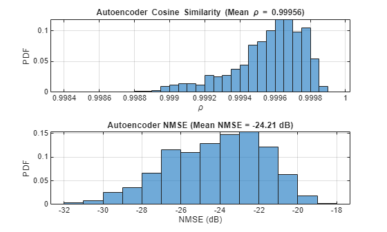
HTestComplex = squeeze(complex(HTestReal(:,:,1,:), HTestReal(:,:,2,:)));
HPredComplex = squeeze(complex(HPredReal(:,:,1,:), HPredReal(:,:,2,:)));
rho = abs(helperComplexCosineSimilarity(HTestComplex, HPredComplex)); % Compute complex cosine similarity
meanRho = mean(rho);
[nmse,meanNmse] = helperCSINMSELossdB(HTestComplex, HPredComplex);    % Compute NMSE
helperPlotMetrics(rho, meanRho, nmse, meanNmse);

metricsTable = table(autoencoderNetwork, compressionFactor, meanNmse, ...
  meanRho, elapsedTime, single(py.csi_feedback_wrapper.info(pyCSINN)), ...
    'VariableNames', {'Model', 'Compression Factor', 'NMSE(dB)', 'Rho', 'InferenceTime', 'NumberOfLearnables'});
disp(metricsTable)

     Model     Compression Factor    NMSE(dB)      Rho      InferenceTime    NumberOfLearnables
    _______    __________________    ________    _______    _____________    __________________

    "CLNet"            4             -24.215     0.99956       6.8655            1.0289e+05    

Save Trained Network

Enable saveNetwork to save the trained model in a PT file with the filename as checkPointName.

saveNetwork = true;
if saveNetwork % Save the trained network
    checkPointName = autoencoderNetwork+string(compressionFactor);
    py.csi_feedback_wrapper.save(trainedNet,checkPointName,autoencoderNetwork, inputLayerSize, compressionFactor);
end

Compare Networks

The following table compares the performance metrics, inference time, and learnable parameters of CLNet across compression factors 4, 16, and 64.

Model	Compression Factor	NMSE(dB)	Rho	Inference Time	Number of Learnables
CLNet	4	-46.639	0.99999	0.14911	1.0289e05
CLNet	16	-44.06	0.99998	0.18851	27538
CLNet	64	-35.524	0.99983	0.15048	8701

Further Exploration

In this example, you train and test the PyTorch network, CLNet, using online training. The CSI feedback autoencoder architecture achieves comparable NMSE and cosine similarity performance across different compression ratios. Adjust the data generation parameters and optimize hyperparameters for your specific use case.

For more information about offline training and throughput analysis, see these examples:

• Offline Training and Testing of PyTorch Model for CSI Feedback Compression

• NR PDSCH Throughput Using Channel State Information Feedback (5G Toolbox)

References

[1] Ji, S., & Li, M. (2021). CLNet: Complex Input Lightweight Neural Network Designed for Massive MIMO CSI Feedback. IEEE Wireless Communications Letters, 10(10), 2318–2322. doi:10.1109/lwc.2021.3100493

Helper Functions

• helperSetupPyenv.m

• helperinstalledlibs.py

• helperLibraryChecker.m

• helperCSIDownloadFiles.m

• helperCSIGenerateData.m

• helperCSIChannelEstimate.m

• helperCSIPreprocessChannelEstimate.m

• helperCSISplitData.m

• CSIFeedback.py

• clnet.py

• csi_feedback_wrapper.py

• helperCSINMSELossdB.m

• helperNMSE.m

• helperComplexCosineSimilarity.m

PyTorch Wrapper Template

You can use your own PyTorch models in MATLAB using the Python interface. The py_wrapper_template.py file provides a simple interface with a predefined API. This example uses the following API set:

• construct_model: returns the PyTorch neural network model

• train: trains the PyTorch model

• setup_trainer: sets up a trainer object for with online training

• train_one_iteration: trains the PyTorch model for one iteration for online training

• validate: validates the PyTorch model for online training

• predict: runs the PyTorch model with the provided input(s)

• save: saves the PyTorch model and metadata

• load: loads the PyTorch model

• info: prints or returns information on the PyTorch model

The Train PyTorch Channel Prediction Models example shows a training workflow and uses the following API set in addition to the one used in this example.

• save_model_weights: saves the PyTorch model weights

• load_model_weights: loads the PyTorch model weights

You can modify the py_wrapper_template.py file. Follow the instruction in the template file to implement the recommended entry points. Delete the entry points that are not relevant to your project. Use the entry point functions as shown in this example to use your own PyTorch models in MATLAB.

Local Functions

function [carrier,channel] = helperCSIGetCarrierAndChannel(dataGenerationInfo)
%helperCSIGetCarrierAndChannel Function to return carrier and channel
%objects based on input parameters
carrier = nrCarrierConfig;
carrier.NSizeGrid = dataGenerationInfo.NSizeGrid;
carrier.SubcarrierSpacing = dataGenerationInfo.SubcarrierSpacing;
waveInfo = nrOFDMInfo(carrier);

% numSubCarriers = dataGenerationInfo.NSizeGrid*12; % 12 subcarriers per RB

samplesPerSlot = ...
  sum(waveInfo.SymbolLengths(1:waveInfo.SymbolsPerSlot));

channel = nrCDLChannel;
channel.DelayProfile = dataGenerationInfo.DelayProfile;
channel.DelaySpread = dataGenerationInfo.RMSDelaySpread;       % s
channel.MaximumDopplerShift = dataGenerationInfo.MaxDoppler;   % Hz
channel.RandomStream = "Global stream";
channel.TransmitAntennaArray.Size = dataGenerationInfo.TxAntennaSize;
channel.ReceiveAntennaArray.Size = dataGenerationInfo.RxAntennaSize;
channel.ChannelFiltering = false;           % No filtering for 
                                            % perfect estimate
channel.NumTimeSamples = samplesPerSlot;    % 1 slot worth of samples
channel.SampleRate = waveInfo.SampleRate;
end

function norm = helperCSIGetNormParams(opt,carrier,channel)
%helperCSIGetNormParams Estimate normalization parameters

numSamples = 1000;

opt.Normalization = false;           % Do not normalize data yet

% Calculate dependent parameters
subcarrierPerRB = 12;
opt.NumSubcarriers = carrier.NSizeGrid*subcarrierPerRB;
channelInfo = info(channel);

if isa(channel,"nrCDLChannel")
  opt.Ntx = channelInfo.NumInputSignals;  % Number of Tx antennas
  opt.Nrx = channelInfo.NumOutputSignals; % Number of Rx antennas
  % Make sure that this is high enough for nrPerfectChannelEstimate to return
  % the full number of symbols worth of channel estimates
  opt.ChannelSampleDensity = 64*4;
else
  opt.Ntx = channelInfo.NumTransmitAntennas;
  opt.Nrx = channelInfo.NumReceiveAntennas;
end

% Calculate the number of frames required to generate these training
% samples. Each slot has Nrx training channel estimates.
numSlots = ceil(numSamples/opt.Nrx);
numFrames = ceil(numSlots/opt.NumSlotsPerFrame);
if numFrames == 1
  % If only one frame is enough, adjust slots per frame
  opt.NumSlotsPerFrame = numSlots;
end

[~,HReal] = helperCSIGenerateData(numFrames,channel,carrier,opt);
norm.MeanVal = mean(HReal,'all');
norm.StdValue = std(HReal,[],'all');
norm.TargetSTDValue = 0.0212;
end

function varargout = helperCSISetBackgroundDataGen(dataGenerationInfo,carrier, ...
                                                   channel,norm, ...
                                                   batchSize)
%helperCSISetBackgroundDataGen Setup background data generation for online
%training

if ~isempty(gcp("nocreate"))
    p = gcp("nocreate");
else
    p = parpool;
end
   
numTrainFutures = p.NumWorkers;
varargout{1}(1:numTrainFutures) = parallel.FevalFuture;
for idx = 1:numTrainFutures
    varargout{1}(idx) = parfeval(@helperCSIGenerateAndSplitData, 2, ...
                                 dataGenerationInfo, carrier, channel, ...
                                 norm, batchSize);
end
end

function [dataFuture,HTReal,HVReal] = helperCSIPrepareDataInParallel(dataGenerationInfo,carrier,channel, ...
                                                                     norm,batchSize,dataFuture)
%helperCSIPrepareDataInParallel Generate data using background processing
[completedIdx,HTReal,HVReal] = fetchNext(dataFuture);
dataFuture(completedIdx) = parfeval(@helperCSIGenerateAndSplitData, 2, ...
                                    dataGenerationInfo, carrier, channel, ...
                                    norm, batchSize);
end

function [HTReal,HVReal] = helperCSIGenerateAndSplitData(opt,carrier,channel,norm,batchSize)
%helperCSIGenerateAndSplitData Generate, split and normalize data for
%online training
numSamples = round(batchSize+0.3*batchSize);

opt.NumSlotsPerFrame = 1;
opt.ResetChannelPerFrame = true;     % Reset after each frame
opt.Normalization = false;           % Do not normalize data yet
opt.Preprocess = true;               % Decimate using
                                     % frequency domain truncation
opt.UseParallel = false;
opt.SaveData = false;
opt.ZeroTimingOffset = false;
opt.Verbose = false;

% Calculate dependent parameters
subcarrierPerRB = 12;
opt.NumSubcarriers = carrier.NSizeGrid*subcarrierPerRB;
channelInfo = info(channel);

if isa(channel,"nrCDLChannel")
  opt.Ntx = channelInfo.NumInputSignals;  % Number of Tx antennas
  opt.Nrx = channelInfo.NumOutputSignals; % Number of Rx antennas
  % Make sure that this is high enough for nrPerfectChannelEstimate to return
  % the full number of symbols worth of channel estimates
  opt.ChannelSampleDensity = 64*4;
else
  opt.Ntx = channelInfo.NumTransmitAntennas;
  opt.Nrx = channelInfo.NumReceiveAntennas;
end

% Calculate the number of frames required to generate these training
% samples. Each slot has Nrx training channel estimates.
numSlots = ceil(numSamples/opt.Nrx);
numFrames = ceil(numSlots/opt.NumSlotsPerFrame);
if numFrames == 1
  % If only one frame is enough, adjust slots per frame
  opt.NumSlotsPerFrame = numSlots;
end

% Data generation
[~,HReal] = helperCSIGenerateData(numFrames,channel,carrier,opt);
[nDelay,nTx,nIQ,nRx,nFrames] = size(HReal);
HReal = reshape(HReal,[nDelay,nTx,nIQ,nRx*nFrames]);

% Split generated data into train and val
splitRatio = [10,3];
[HTReal, HVReal] = helperCSISplitData(HReal,splitRatio);

% Normalize the data
[HTReal, HVReal] = helperCSINormalizeOnlineData(norm, HTReal, HVReal);
end

function varargout = helperCSINormalizeOnlineData(norm,varargin)
%helperCSINormalizeOnlineData Normalize the input based on the NORM
%parameters
numInputs = nargin-1;
varargout = cell(1,numInputs);
for i=1:numInputs
    varargout{i} = (varargin{i}-norm.MeanVal)/norm.StdValue*norm.TargetSTDValue+0.5;
end
end

function helperPlotMetrics(rho,meanRho,nmse,meanNmse)
%helperPlotMetrics Plot the histograms for RHO and NMSE values
figure
tiledlayout(2,1)
nexttile
histogram(rho,"Normalization","probability")
grid on
title(sprintf("Autoencoder Cosine Similarity (Mean \\rho = %1.5f)", ...
    meanRho))
xlabel("\rho"); ylabel("PDF")
nexttile
histogram(nmse,"Normalization","probability")
grid on
title(sprintf("Autoencoder NMSE (Mean NMSE = %1.2f dB)",meanNmse))
xlabel("NMSE (dB)"); ylabel("PDF")
end