looptuneSetup

Convert tuning setup for looptune to tuning setup for systune

Syntax

[T0,SoftReqs,HardReqs,sysopt] = looptuneSetup(looptuneInputs)

Description

[T0,SoftReqs,HardReqs,sysopt] = looptuneSetup(looptuneInputs) converts a tuning setup for looptune into an equivalent tuning setup for systune. The argument looptuneInputs is a sequence of input arguments for looptune that specifies the tuning setup. For example,

[T0,SoftReqs,HardReqs,sysopt] = looptuneSetup(G0,C0,wc,Req1,Req2,loopopt)

generates a set of arguments such that looptune(G0,C0,wc,Req1,Req2,loopopt) and systune(T0,SoftReqs,HardReqs,sysopt) produce the same results.

Use this command to take advantage of additional flexibility that systune offers relative to looptune. For example, looptune requires that you tune all channels of a MIMO feedback loop to the same target bandwidth. Converting to systune allows you to specify different crossover frequencies and loop shapes for each loop in your control system. Also, looptune treats all tuning requirements as soft requirements, optimizing them but not requiring that any constraint be exactly met. Converting to systune allows you to enforce some tuning requirements as hard constraints, while treating others as soft requirements.

You can also use this command to probe into the tuning requirements used by looptune.

Note

When tuning Simulink^® models through an slTuner interface, use looptuneSetup (Simulink Control Design) for slTuner.

Examples

Convert looptune Problem into systune Problem

Convert a set of looptune inputs into an equivalent set of inputs for systune.

Suppose you have a numeric plant model, G0, and a tunable controller model, C0. Suppose also that you used looptune to tune the feedback loop between G0 and C0 to within a bandwidth of wc = [wmin,wmax]. Convert these variables into a form that allows you to use systune for further tuning.

[T0,SoftReqs,HardReqs,sysopt] = looptuneSetup(C0,G0,wc);

The command returns the closed-loop system and tuning requirements for the equivalent systune command, systune(CL0,SoftReqs,HardReqs,sysopt). The arrays SoftReqs and HardReqs contain the tuning requirements implicitly imposed by looptune. These requirements enforce the target bandwidth and default stability margins of looptune.

If you used additional tuning requirements when tuning the system with looptune, add them to the input list of looptuneSetup. For example, suppose you used a TuningGoal.Tracking requirement, Req1, and a TuningGoal.Rejection requirement, Req2. Suppose also that you set algorithm options for looptune using looptuneOptions. Incorporate these requirements and options into the equivalent systune command.

[T0,SoftReqs,HardReqs,sysopt] = looptuneSetup(C0,G0,wc,Req1,Req2,loopopt);

The resulting arguments allow you to construct an equivalent tuning problem for systune. In particular, [~,C] = looptune(C0,G0,wc,Req1,Req2,loopopt) yields the same result as the following commands.

T = systune(T0,SoftReqs,HardReqs,sysopt);
C = setBlockValue(C0,T);

Convert Distillation Column Problem for Tuning With systune

Set up the following control system for tuning with looptune. Then convert the setup to a systune problem and examine the results. These results reflect the structure of the control system model that looptune tunes. The results also reflect the tuning requirements implicitly enforced when tuning with looptune.

For this example, the 2-by-2 plant G is represented by:

$$G\left(s\right)=\frac{1}{75s+1}\left[\begin{array}{cc}87.8& -86.4\\ 108.2& -109.6\end{array}\right].$$

The fixed-structure controller, C, includes three components: the 2-by-2 decoupling matrix D and two PI controllers PI_L and PI_V. The signals r, y, and e are vector-valued signals of dimension 2.

Build a numeric model that represents the plant and a tunable model that represents the controller. Name all inputs and outputs as in the diagram, so that looptune and looptuneSetup know how to interconnect the plant and controller via the control and measurement signals.

s = tf('s');
G = 1/(75*s+1)*[87.8 -86.4; 108.2 -109.6];
G.InputName = {'qL','qV'};
G.OutputName = {'y'};

D = tunableGain('Decoupler',eye(2));
D.InputName = 'e';
D.OutputName = {'pL','pV'};
PI_L = tunablePID('PI_L','pi');
PI_L.InputName = 'pL';
PI_L.OutputName = 'qL';
PI_V = tunablePID('PI_V','pi'); 
PI_V.InputName = 'pV';
PI_V.OutputName = 'qV'; 
sum1 = sumblk('e = r - y',2);
C0 = connect(PI_L,PI_V,D,sum1,{'r','y'},{'qL','qV'});

This system is now ready for tuning with looptune, using tuning goals that you specify. For example, specify a target bandwidth range. Create a tuning requirement that imposes reference tracking in both channels of the system with a response time of 15 s, and a disturbance rejection requirement.

wc = [0.1,0.5];
TR = TuningGoal.Tracking('r','y',15,0.001,1);
DR = TuningGoal.Rejection({'qL','qV'},1/s);
DR.Focus = [0 0.1];

[G,C,gam,info] = looptune(G,C0,wc,TR,DR);

Final: Peak gain = 1, Iterations = 42
Achieved target gain value TargetGain=1.

looptune successfully tunes the system to these requirements. However, you might want to switch to systune to take advantage of additional flexibility in configuring your problem. For example, instead of tuning both channels to a loop bandwidth inside wc, you might want to specify different crossover frequencies for each loop. Or, you might want to enforce the tuning requirements TR and DR as hard constraints, and add other requirements as soft requirements.

Convert the looptune input arguments to a set of input arguments for systune.

[T0,SoftReqs,HardReqs,sysopt] = looptuneSetup(G,C0,wc,TR,DR);

This command returns a set of arguments you can provide to systune for equivalent results to tuning with looptune. In other words, the following command is equivalent to the previous looptune command.

[T,fsoft,ghard,info] = systune(T0,SoftReqs,HardReqs,sysopt);

Final: Peak gain = 1, Iterations = 42
Achieved target gain value TargetGain=1.

Examine the arguments returned by looptuneSetup.

T0

Generalized continuous-time state-space model with 0 outputs, 2 inputs, 4 states, and the following blocks:
  APU_: Analysis point, 2 channels, 1 occurrences.
  APY_: Analysis point, 2 channels, 1 occurrences.
  Decoupler: Tunable 2x2 gain, 1 occurrences.
  PI_L: Tunable PID controller, 1 occurrences.
  PI_V: Tunable PID controller, 1 occurrences.

Type "ss(T0)" to see the current value and "T0.Blocks" to interact with the blocks.

The software constructs the closed-loop control system for systune by connecting the plant and controller at their control and measurement signals, and inserting a two-channel AnalysisPoint block at each of the connection locations, as illustrated in the following diagram.

When tuning the control system of this example with looptune, all requirements are treated as soft requirements. Therefore, HardReqs is empty. SoftReqs is an array of TuningGoal requirements. These requirements together enforce the bandwidth and margins of the looptune command, plus the additional requirements that you specified.

SoftReqs

SoftReqs=5×1 object
  5x1 heterogeneous SystemLevel (LoopShape, Tracking, Rejection, ...) array with properties:

    Models
    Openings
    Name

Examine the first entry in SoftReqs.

SoftReqs(1)

ans = 
  LoopShape with properties:

       LoopGain: [1x1 zpk]
       CrossTol: 0.3495
          Focus: [0 Inf]
      Stabilize: 1
    LoopScaling: 'on'
       Location: {2x1 cell}
         Models: NaN
       Openings: {0x1 cell}
           Name: 'Open loop CG'

looptuneSetup expresses the target crossover frequency range wc as a TuningGoal.LoopShape requirement. This requirement constrains the open-loop gain profile to the loop shape stored in the LoopGain property, with a crossover frequency and crossover tolerance (CrossTol) determined by wc. Examine this loop shape.

viewGoal(SoftReqs(1))

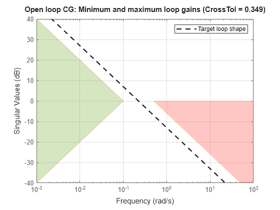
The target crossover is expressed as an integrator gain profile with a crossover between 0.1 and 0.5 rad/s, as specified by wc. If you want to specify a different loop shape, you can alter this TuningGoal.LoopShape requirement before providing it to systune.

looptune also tunes to default stability margins that you can change using looptuneOptions. For systune, stability margins are specified using TuningGoal.Margins requirements. Here, looptuneSetup has expressed the default stability margins of looptune as soft TuningGoal.Margins requirements. For example, examine the fourth entry in SoftReqs.

SoftReqs(4)

ans = 
  Margins with properties:

      GainMargin: 7.6000
     PhaseMargin: 45
    ScalingOrder: 0
           Focus: [0 Inf]
        Location: {2x1 cell}
          Models: NaN
        Openings: {0x1 cell}
            Name: 'Margins at plant inputs'

The last entry in SoftReqs is a similar TuningGoal.Margins requirement constraining the margins at the plant outputs. looptune enforces these margins as soft requirements. If you want to convert them to hard constraints, pass them to systune in the input vector HardReqs instead of the input vector SoftReqs.

Input Arguments

looptuneInputs — Plant, controller, and requirement inputs to looptune

valid looptune input sequence

Plant, controller, and requirement inputs to looptune, specified as a valid looptune input sequence. For more information about the arguments in a valid looptune input sequence, see the looptune reference page.

Output Arguments

T0 — Closed-loop control system model

generalized state-space model

Closed-loop control system model for tuning with systune, returned as a generalized state-space genss model. To compute T0, the plant, G0, and the controller, C0, are combined in the feedback configuration of the following illustration.

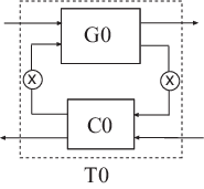
The connections between C0 and G0 are determined by matching signals using the InputName and OutputName properties of the two models. In general, the signal lines in the diagram can represent vector-valued signals. AnalysisPoint blocks, indicated by X in the diagram, are inserted between the controller and the plant. This allows definition of open-loop and closed-loop requirements on signals injected or measured at the plant inputs or outputs. For example, the bandwidth wc is converted into a TuningGoal.LoopShape requirement that imposes the desired crossover on the open-loop signal measured at the plant input.

For more information on the structure of closed-loop control system models for tuning with systune, see the systune reference page.

SoftReqs — Soft tuning requirements

vector of TuningGoal requirement objects

Soft tuning requirements for tuning with systune, specified as a vector of TuningGoal requirement objects.

looptune expresses most of its implicit tuning requirements as soft tuning requirements. For example, a specified target loop bandwidth is expressed as a TuningGoal.LoopShape requirement with integral gain profile and crossover at the target frequency. Additionally, looptune treats all of the explicit requirements you specify (Req1,...ReqN) as soft requirements. SoftReqs contains all of these tuning requirements.

HardReqs — Hard tuning requirements

vector of TuningGoal requirement objects

Hard tuning requirements (constraints) for tuning with systune, specified as a vector of TuningGoal requirement objects.

Because looptune treats most tuning requirements as soft requirements, HardReqs is usually empty. However, if you change the default MaxFrequency option of the looptuneOptions set, loopopt, then this requirement appears as a hard TuningGoal.Poles constraint.

sysopt — Algorithm options for systune tuning

systuneOptions options set

Algorithm options for systune tuning, specified as a systuneOptions options set.

Some of the options in the looptuneOptions set, loopopt, are expressed as hard or soft requirements that are returned in HardReqs and SoftReqs. Other options correspond to options in the systtuneOptions set.

Alternatives

When tuning Simulink using an slTuner, interface, convert a looptune problem to systune using looptuneSetup (Simulink Control Design) for slTuner.

Version History

Introduced in R2013b