Direction-of-Arrival Estimation Using Deep Learning

This example demonstrates a deep learning approach for direction-of-arrival (DOA) estimation. [1] The deep DOA estimator predicts angular directions directly from the sample covariance matrix, addressing the challenges of parameter sensitivity and reduced performance under extreme noise conditions often encountered in traditional methods.

Data set Preparation

The data set for this example is generated using simulations using Phased Array System Toolbox™ simulations. Data is generated using a uniform linear array (ULA) with 8 receivers over multiple SNR scenarios to train the model to work effectively over a rich range of noise powers. Each data set sample consists of 200 received signal snapshots. Noise power is varied across four levels: 0, 1, 2, and 5 times the signal power. The data is generated using one and two signal sources, thus enabling the model to identify one or two sources without requiring prior knowledge. The deep learning model itself does not impose a limit on the maximum number of sources. However, more sources require additional training data and longer training time. For simplicity, this example considers only cases with 1 or 2 sources to demonstrate the approach.

fc = 300e6;
lambda = physconst("LightSpeed")/fc;
ula = phased.ULA(NumElements=8,ElementSpacing=lambda/2);
nsanpshots = 200;

One classic method for DOA estimation is the Multiple Signal Classification (MUSIC) algorithm. The algorithm a power expression dependent on the arrival angle, known as the MUSIC pseudospectrum. The estimated directions of arrival are the angles where the pseudospectrum has peaks.

Similar to the MUSIC algorithm, the deep learning model in this example uses a discretization on-grid approach to resolve angles within the grid resolution. During training, the grid resolution is defined as 1 degree, covering a range from –90 degrees to 90 degrees, resulting in 181 grid points. Increasing the number of grid points improves the discretization resolution but requires more training data to support a larger model, leading to higher computational costs.

angleGrid = -90:1:90;

Use the helperGenerateTrainData function to generate the data set by simulating the received signals at the ULA under the specified conditions. Fix the random seed for reproducibility.

rng("default")
[signalsTrain,scovsTrain,anglesTrain] = helperGenerateTrainData(NoisePower=[0,1,2,5], ...
    Shuffle=true, ...
    ULA=ula, ...
    Nsnapshots=nsanpshots);

Split the covariance matrix into real and imaginary components to make it compatible with convolutional neural networks, which work only with real-valued data.

ndata = length(anglesTrain);
sigCov = zeros([size(signalsTrain,2) size(signalsTrain,2) 1 size(signalsTrain,3)]);
sigCov(:,:,1,:) = real(scovsTrain);
sigCov(:,:,2,:) = imag(scovsTrain);

The sigCov matrix is structured as a 4-D array with dimensions 8-by-8-by-2-by-65884. The first two dimensions, both of which are 8, correspond to the size of the covariance matrix, which is treated as the height and width of an image when used as input to the convolutional neural network. The third dimension, 2, represents the channel dimension, where the real and imaginary components of the covariance matrix are split into separate channels. Finally, the fourth dimension, 65884, corresponds to the batch dimension, equal to the total number of observations.

whos sigCov

  Name        Size                      Bytes  Class     Attributes

  sigCov      8x8x2x65884            67465216  double              

Create a logical matrix where rows represent angles in the angleGrid and columns correspond to observations. A value of 1 in a row indicates the presence of that angle for the corresponding signal. Use this matrix as the ground truth for training the deep learning model.

anglesBinaryVec = zeros([length(angleGrid) size(signalsTrain,3) ]);
for ii = 1:ndata
    angleSet = anglesTrain{ii};
    anglesBinaryVec(:,ii) = ismember(angleGrid,angleSet);
end

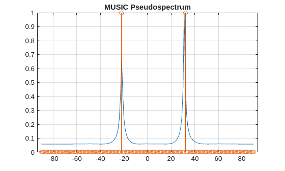
Apply the MUSIC algorithm to a signal in the dataset, setting it to automatically detect the number of signals. The plot compares the MUSIC estimates with the actual angle locations.

ii = randi(ndata);
signal = signalsTrain(:,:,ii);
scanAngles = linspace(-90,90,181);
musicEstimator = phased.MUSICEstimator(SensorArray=ula, ...
    OperatingFrequency=fc, ...
    ScanAngles=scanAngles, ...
    DOAOutputPort=true, ...
    NumSignalsSource="Auto");
ymusic = musicEstimator(signal);

plot(scanAngles,ymusic./max(ymusic))
hold on
stem(scanAngles,anglesBinaryVec(:,ii))
hold off
title("MUSIC Pseudospectrum")
grid on 
box on

DOA Estimation Using Deep Learning

Deep DOA Estimator Model

Compared to traditional methods, deep learning approaches enhance robustness in the presence of noise and show greater resilience to a relatively small number of snapshots. Moreover, deep learning methods can estimate the number of sources more accurately. This example specifically models the DOA problem as a multilabel classification task, identifying whether a signal source arriving from a specific angle in the grid. A convolutional neural network (CNN) is trained to predict DOAs across all SNRs. The CNN uses covariance matrices, split into their real and imaginary parts, as input. The network produces a probability vector instead of a traditional spectrum. Each element in the probability vector represents the likelihood of a source being present at the corresponding direction angle.

When the number of sources, K, is known, the top K peaks in the probability vector are selected as the source directions. When the number of sources is unknown, a thresholding method is applied to identify peaks in the probability vector. Peaks that exceed the predefined threshold are considered as sources, and their positions indicate the corresponding directions. The number of peaks above the threshold determines the estimated number of sources.

Define the CNN architecture.

kern_size1 = 3;
kern_size2 = 2;
m = size(scovsTrain,1);
r = length(angleGrid);
layers = [
    imageInputLayer([m m 2],Normalization="none")

    convolution2dLayer(kern_size1, 256, Padding="same")
    batchNormalizationLayer()
    reluLayer()

    convolution2dLayer(kern_size2, 256, Padding="same")
    batchNormalizationLayer()
    reluLayer()

    convolution2dLayer(kern_size2, 256, Padding="same")
    batchNormalizationLayer()
    reluLayer()

    convolution2dLayer(kern_size2, 256, Padding="same")
    batchNormalizationLayer()
    reluLayer()

    fullyConnectedLayer(4096)
    reluLayer()
    dropoutLayer(0.3)

    fullyConnectedLayer(2048)
    reluLayer()
    dropoutLayer(0.3)

    fullyConnectedLayer(1024)
    reluLayer()
    dropoutLayer(0.3)

    fullyConnectedLayer(r,WeightsInitializer="glorot")
    sigmoidLayer()
    ];

Split the data set into training and validation sets. The validation set is specifically used to determine the optimal threshold for handling cases with an unknown number of sources.

N = ndata;
trainIdx = 1:floor(0.8*N);
validIdx = floor(0.9*N)+1:N;

trainData = dlarray(sigCov(:,:,:,trainIdx),"SSCB");
trainLabels = dlarray(anglesBinaryVec(:,trainIdx),"CB");

validData = dlarray(sigCov(:,:,:,validIdx),"SSCB");
validLabels = dlarray(anglesBinaryVec(:,validIdx),"CB");

Train the Network

In the loss function, assign a higher weight to locations where sources exist to enable the model to learn more effectively. Specifically, y is the predicted probability vector, and t is the ground truth binary vector indicating where sources are present. The operation t*10+1 increases the weight of locations where sources exist by setting their weight to 11, while non-source locations remain at 1. This ensures the model focuses more on correctly predicting source locations during training.

function loss = customLoss(y,t) %#ok<DEFNU>
    loss = crossentropy(y,t,t*10+1,ClassificationMode="multilabel"); 
end

metric = accuracyMetric(ClassificationMode="multilabel");

options = trainingOptions("adam", ...
    InitialLearnRate=1e-4, ...
    MaxEpochs=2000, ...
    MiniBatchSize=5000, ...
    Shuffle="every-epoch", ...
    Verbose=true, ...
    Plots="training-progress", ...
    ExecutionEnvironment="auto", ...
    Metrics=metric, ...
    OutputNetwork="last-iteration");

Train the model using the customized cross-entropy loss function. You can skip this training by downloading a pretrained network using the selector below. If you want to train the network as the example runs, set trainNow to true. If you want to skip the training steps and download a MAT file containing the pretrained network, set trainNow to false.

trainNow = false;
if trainNow 
    deepDOAEstimator = trainnet(trainData,trainLabels,layers,@(y,t)customLoss(y,t),options); %#ok<UNRCH>
else
    datasetZipFile = matlab.internal.examples.downloadSupportFile('SPT','data/deepDOACNNModel.zip');
    datasetFolder = fullfile(fileparts(datasetZipFile),'deepDOACNNModel');
    if ~exist(datasetFolder,'dir')     
        unzip(datasetZipFile,datasetFolder);
    end
    file = load(fullfile(datasetFolder,"deepDOACNNModel.mat"));
    deepDOAEstimator = file.deepDOAEstimator;
end

After training, randomly select an observation from the validation set and compare the MUSIC estimator's pseudospectrum with the deep DOA estimator's learned target probability over angles.

Use the minibatchpredict function to predict the angle probability vector using the trained deep DOA estimator. The dotted lines on the plots mark the true angle locations.

rng("default")
idxList = randi(length(validIdx),[1,4]);
figure(Position=[0 0 2000 500])
tiledlayout(2,4)
colors = lines(2);
for ii = 1:length(idxList)
    idx = validIdx(idxList(ii));
    signal = signalsTrain(:,:,idx);
    [ymusic,angs] = musicEstimator(signal);
    scov = sigCov(:,:,:,idx);
    probVec = minibatchpredict(deepDOAEstimator,dlarray(scov,"SSCB"));
   
    nexttile(ii)
    plot(scanAngles,ymusic./max(ymusic))
    title("MUSIC Pseudospectrum ")
    xline(anglesTrain{idx},"--",Color=colors(2,:))
    grid on 
    box on
    
    nexttile(ii+4)
    plot(angleGrid,probVec)
    xline(anglesTrain{idx},"--",Color=colors(2,:))
    title("Deep DOA Estimator Probability Vector")
    xlabel("Angle")
    ylabel("Probability")
    box on 
    grid on
end

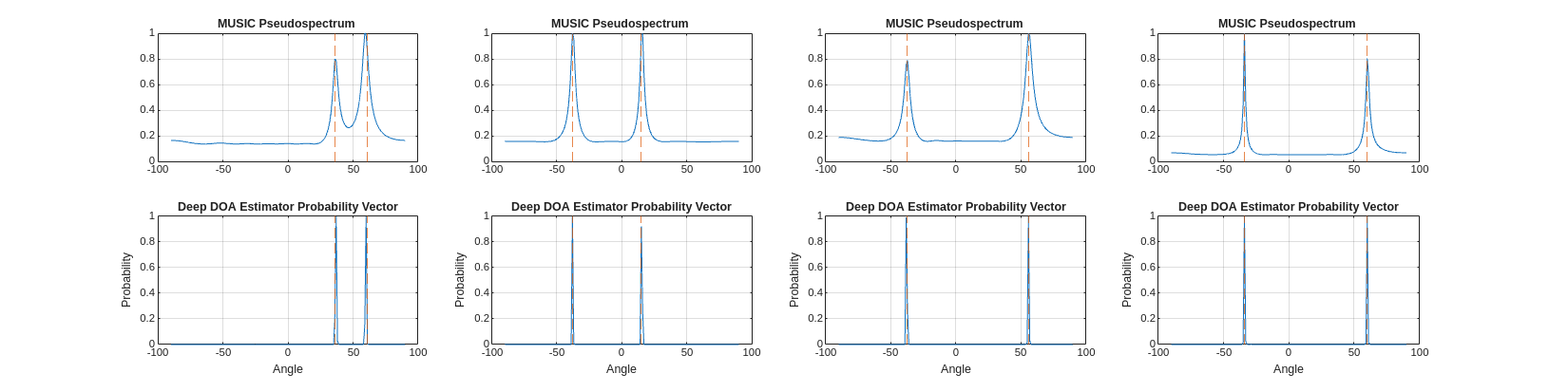
Both methods exhibit distinct peaks at the directions where sources exist. However, the peaks from the deep DOA estimator are sharper.

Determine Optimal Threshold for Unknown Number of Sources

To enable usage when the number of sources is unknown, the deep DOA estimator requires a probability threshold to determine whether a probability peak is large enough to indicate the presence of a signal source.

Use validation data to identify the optimal threshold by sweeping through values between 0 and 1. For each threshold, the number of detected sources is compared to the actual number of sources in the data. Accuracy is defined as the percentage of cases where the detected number matches the actual number. The threshold that maximizes this accuracy is selected to optimize performance.

validProbVec = minibatchpredict(deepDOAEstimator,dlarray(sigCov(:,:,:,validIdx),"SSCB"));
thresholds = linspace(0,1,200); 
accuracies = zeros(size(thresholds));

nsourcesAct = cellfun(@(x)numel(x),anglesTrain(validIdx),UniformOutput=true);
validProbVecNorm = extractdata(validProbVec);

peaksArray = cell(1,size(validProbVec,2));
for col = 1:size(validProbVec,2)
    peaksArray{col} = findpeaks(validProbVecNorm(:,col),MinPeakHeight=0.05);
end
for i = 1:length(thresholds)
    threshold = thresholds(i);
    nsourcesEst = cellfun(@(peaks)numel(peaks(peaks>threshold)),peaksArray)';
    accuracies(i) = sum(nsourcesAct==nsourcesEst)/numel(nsourcesAct);
end

[maxAccuracy, bestIdx] = max(accuracies);
bestThreshold = thresholds(bestIdx);

figure
plot(thresholds,accuracies,LineWidth=2)
xline(bestThreshold,"--",LineWidth=2,Color=colors(2,:))
xlabel("Threshold")
ylabel("Accuracy")
title(["Threshold vs. Accuracy" ...
    "Max Accuracy = "+maxAccuracy ...
    "Optimal Threshold = "+bestThreshold])
ylim([0 1])
grid on
box on

Performance Evaluation of Deep DOA Estimator Under Various Conditions

To evaluate fairly the generalization ability of the deep DOA estimator, the test data is obtained from newly generated signals using settings that are different than those used to generate the training data. These differences include varying the number of snapshots, introducing broader SNR ranges, and incorporating off-grid angles. The results are compared with the traditional MUSIC estimator under various conditions.

Performance Evaluation with Known Number of Sources Scenario

First, evaluate the performance of the Deep DOA estimator and the MUSIC estimator under the condition where the number of sources is known. For a fixed number of sources case, the MUSIC estimator is also configured with a given NumSignalsSource parameter. The NumSignals is set to 2 for subsequent use.

musicEstimator2Sources = phased.MUSICEstimator(SensorArray=ula, ...
    OperatingFrequency=fc, ...
    ScanAngles=scanAngles, ...
    DOAOutputPort=true, NumSignalsSource="Property", NumSignals=2);

To intuitively compare the performance differences between the two estimators, first consider a scenario with two signal sources having a fixed angular separation of 10 degrees. The direction of the first signal source varies within the range of –90 degrees to 90 degrees. The SNR is set to 0 dB, meaning the noise power is equal to the signal power, and the number of snapshots is 500. To make the scenario more realistic, the angles are off-grid. An off-grid angle means that, unlike the angles used in the training data, the testing angles are not all integers. Because of this, a periodic error from rounding should be expected for both estimators.

angleDiff = 10;
angleSweepStepSize = 0.73;
angleList = -90:angleSweepStepSize:90 - angleDiff;
nAnglePairs = length(angleList);

nsamples = 1;
signalTest = cell(nAnglePairs*nsamples,1);
scovTest = cell(nAnglePairs*nsamples,1);
anglesTest = cell(nAnglePairs*nsamples,1);

n = 0;
for ii = 1:nAnglePairs
    anglePair = [angleList(ii) angleList(ii)+angleDiff];
    n = n+1;
    [signal,scov,angle] = helperGenerateTestData( ...
        SourceAngles=anglePair, ...
        NoisePower=1, ...
        NumSnapshots=500,ULA=ula);
    signalTest{n} = signalTest;
    scovTest{n} = cat(3,real(scov),imag(scov));
    anglesTest{n} = anglePair;
end

Estimate DOA using the deep DOA estimator, which can process an entire batch of observations. Use the helperEstimateAngles function to extract angles from the probability vectors generated by the deepDOAEstimator.

scovTestMat = cat(4,scovTest{:});
probVec = minibatchpredict(deepDOAEstimator,dlarray(scovTestMat,"SSCB"));
detectedAnglesNet = helperEstimateAngles(probVec,angleGrid,NumSignalsSource=2);

Estimate DOA using the MUSIC DOA estimator.

detectedAnglesMUSIC = cell(length(signalTest),1);

for ii = 1:length(signalTest)
    covmat = scovTest{ii};
    covmat = covmat(:,:,1)+1j*covmat(:,:,2);
    doas = musicdoa(covmat,2,ScanAngles=angleGrid);
    detectedAnglesMUSIC{ii} = sort(doas);
end

Plot and compare the angles estimated by the two estimators. The plots on the left display the locations of the actual angle pairs (indicated with dot markers) alongside the estimated angle pairs (indicated with cross markers). The plots on the right illustrate the corresponding angle errors, showcasing the deviations between the ground truth and the estimations for each method.

helperPlotAngleSweepTest(anglesTest,detectedAnglesMUSIC,detectedAnglesNet)

It can be observed that in the middle range, –60 degrees to 60 degrees, both estimators perform similarly, with some rounding-induced errors. However, near the edges close to ±90 degrees, MUSIC estimator's performance deteriorates rapidly, while the deepDOAEstimator maintains relatively stable estimation accuracy.

Performance Comparison Across SNR Scenarios

To systematically and quantitatively compare the performance of the two estimators, vary a single parameter while keeping others fixed, and plot the performance trends of both estimators as the parameter changes.

First, select different SNR scenarios by adjusting the ratio of noise power to signal power. In this case, SNR is varied from –15 dB to 1 dB, while the SNR of the training data is always higher than –7 dB. The angular spacing is fixed at 5 degrees, specifically choosing angles of 10 and 15 degrees, which are close to the center of angle grid. The number of snapshots is set to 500. For each specific configuration, generate 500 observations to minimize errors caused by randomness.

SNRList = -15:2:1;
noisePowerList = db2pow(-SNRList);
nsamples = 500;
nSettings = length(noisePowerList);
signalTest = cell(nSettings*nsamples,1);
scovTest = cell(nSettings*nsamples,1);
anglesTest = cell(nSettings*nsamples,1);
n = 0;
for ii = 1:nSettings
    noisePower = noisePowerList(ii);
    for jj = 1:nsamples
        n = n+1;
        [signal,scov,angles] = helperGenerateTestData( ...
            SourceAngles=[10,15], ...
            NoisePower=noisePower, ...
            NumSnapshots=500,ULA=ula);
        signalTest{n} = signal;
        scovTest{n} = cat(3,real(scov),imag(scov));
        anglesTest{n} = angles{:};
    end
end

Estimate DOA using the deep MUSIC estimator.

detectedAnglesMUSIC = cell(length(anglesTest),1);
for ii = 1:length(signalTest)
    signal = signalTest{ii};
    [~,ang] = musicEstimator2Sources(signal);
    detectedAnglesMUSIC{ii} = sort(ang);
end

Estimate DOA using the deep DOA estimator.

scovTestSNRTensor = dlarray(cat(4,scovTest{:}),"SSCB");
probVec = minibatchpredict(deepDOAEstimator,scovTestSNRTensor);
detectedAnglesDeep = helperEstimateAngles(probVec,angleGrid,NumSignalsSource=2);

Calculate the average angular estimation error for both methods.

errorDeep = cellfun(@(x,y)sum(abs(x-y)),detectedAnglesDeep,anglesTest);
errorDeep = reshape(errorDeep,nsamples,[]);
errorDeep = mean(errorDeep,1);

errorMUSIC = cellfun(@(x,y)sum(abs(x-y)),detectedAnglesMUSIC,anglesTest);
errorMUSIC = reshape(errorMUSIC,nsamples,[]);
errorMUSIC = mean(errorMUSIC,1);

figure
plot(SNRList,errorMUSIC)
hold on
plot(SNRList,errorDeep)
hold off
grid on
box on
ylabel("Error (degrees)")
xlabel("SNR (dB)")
title("Estimation Error Across SNR Levels")
legend(["MUSIC" "Deep DOA Estimator"],Location="best")
xlim([-15 1])

Both methods accurately estimate angles at high SNR levels, but the deep DOA estimator maintains relatively good accuracy even under low SNR conditions. Even under SNR conditions lower than those in the training data, the deep DOA estimator remains stable, demonstrating strong generalization ability across different SNR scenarios.

Performance Comparison Across Snapshots

Next, test the impact of different numbers of snapshots. Fix the SNR at 0 dB while keeping other settings unchanged. The number of snapshots is varied from 50 to 500.

numSnapshotsList = 500:-50:50;
nsamples = 500;
nSettings = length(numSnapshotsList);
signalTest = cell(nSettings*nsamples,1);
scovTest = cell(nSettings*nsamples,1);
anglesTest = cell(nSettings*nsamples,1);
n=0;
for ii = 1:nSettings
    numSnapshots = numSnapshotsList(ii);
    for jj = 1:nsamples
        n = n+1;
        [signal,scov,angles] = helperGenerateTestData(SourceAngles=[10,15], ...
            NoisePower=1, ...
            NumSnapshots=numSnapshots, ...
            ULA=ula);
        signalTest{n} = signal;
        scovTest{n} = cat(3,real(scov),imag(scov));
        anglesTest{n} = angles{:};
    end
end

Estimate DOA using the deep MUSIC estimator.

detectedAnglesMUSIC = cell(length(signalTest),1);
for ii = 1:length(signalTest)
    signal = signalTest{ii};
    [~,ang] = musicEstimator2Sources(signal);
    detectedAnglesMUSIC{ii} = sort(ang);
end

Estimate DOA using the deep DOA estimator.

scovTestSNRTensor = dlarray(cat(4,scovTest{:}),"SSCB");
probVec = minibatchpredict(deepDOAEstimator,scovTestSNRTensor);
detectedAnglesDeep = helperEstimateAngles(probVec,angleGrid,NumSignalsSource=2);

Calculate the average angular estimation error for both methods.

errorDeep = cellfun(@(x,y)sum(abs(x-y)),detectedAnglesDeep,anglesTest);
errorDeep = reshape(errorDeep,nsamples,[]);
errorDeep = mean(errorDeep,1);

errorMUSIC = cellfun(@(x,y)sum(abs(x-y)),detectedAnglesMUSIC,anglesTest);
errorMUSIC = reshape(errorMUSIC,nsamples,[]);
errorMUSIC = mean(errorMUSIC,1);

figure
plot(numSnapshotsList,errorMUSIC)
hold on
plot(numSnapshotsList,errorDeep)
hold off
grid on
box on
ylabel("Error (degrees)")
xlabel("Snapshots")
title("Estimation Error Across Snapshots")
legend(["MUSIC","Deep DOA Estimator"],Location="best")

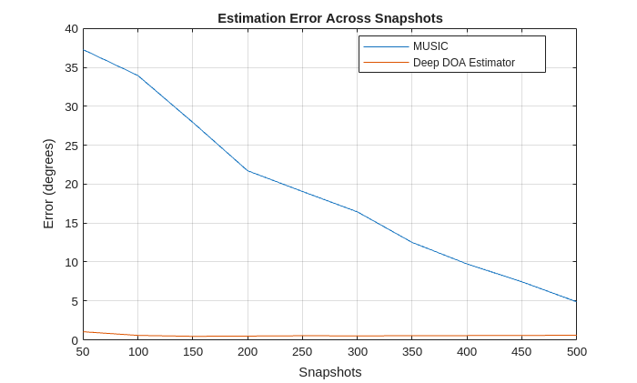
The deep DOA estimator, despite being trained on data with only 200 snapshots, consistently has stable and high-accuracy performance across testing scenarios with varying numbers of snapshots.

Performance Evaluation with Unknown Number of Sources

The next step is to test the scenario with an unknown number of sources. In this case, the primary focus is on evaluating whether both methods can accurately estimate the number of sources.

Randomly generate 500 observations each for scenarios with 1 and 2 signal sources to test the performance of the two estimators.

randomPairs = randi([-90,90],500,2);
randomSingles = randi([-90,90],500,1);
angleList = [mat2cell(randomPairs,ones(500,1),2);num2cell(randomSingles)];
n=0;
nSettings = length(angleList);
nsamples = 1;
signalTest = cell(nSettings*nsamples,1);
scovTest = cell(nSettings*nsamples,1);
anglesTest = cell(nSettings*nsamples,1);
for ii = 1:nSettings
    angles = angleList{ii};
    for jj = 1:nsamples
        n = n+1;
        [signal,scov,angle] = helperGenerateTestData(SourceAngles=angles,NoisePower=2,NumSnapshots=500);
        signalTest{n} = signal;
        scovTest{n} = cat(3,real(scov),imag(scov));
        anglesTest{n} = angle{:};
    end
end

Estimate DOA using the deep DOA estimator. In this case, use the threshold method to determine the actual signal source arrival angles. The threshold is set to the optimal value computed earlier using the validation data.

scovTestSNRTensor = cat(4,scovTest{:});
probVec = minibatchpredict(deepDOAEstimator,dlarray(scovTestSNRTensor,"SSCB"));
detectedAnglesNet = helperEstimateAngles(probVec,angleGrid,Threshold=bestThreshold);

When the number of sources is unknown, redefine the MUSIC estimator with NumSignalsSource set to "Auto". By default, the MUSIC estimator uses the Akaike Information Criterion method to estimate the number of sources.

musicEstimatorAutoSources = phased.MUSICEstimator(SensorArray=ula, ...
    OperatingFrequency=fc, ...
    ScanAngles=scanAngles, ...
    DOAOutputPort=true, ...
    NumSignalsSource="Auto");

Estimate DOA using the MUSIC estimator.

detectedAnglesMUSIC = cell(length(signalTest),1);
for ii = 1:length(signalTest)
    signal = signalTest{ii};
    [~, ang] = musicEstimatorAutoSources(signal);
    detectedAnglesMUSIC{ii} = sort(ang);
end

Compare the accuracy of source number estimation between the two methods.

helperPlotConfusionChart(detectedAnglesMUSIC,detectedAnglesNet,anglesTest)

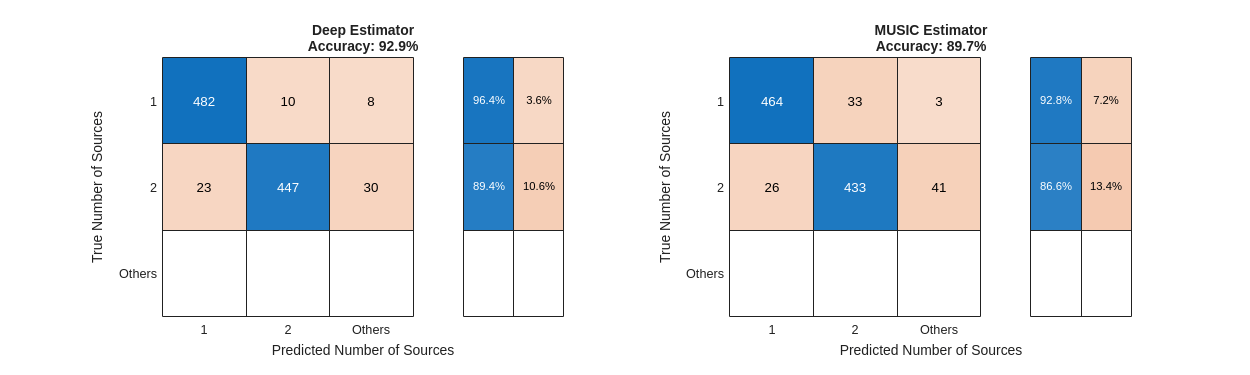
Compared to the MUSIC estimator, the deep DOA estimator achieves better performance on detecting the number of sources.

Summary

This example demonstrates how to model and solve the DOA problem using a deep learning approach. Through a series of tests, it highlights that the deep DOA estimator outperforms the traditional MUSIC algorithm, particularly in scenarios with low SNR, limited snapshots, and unknown number of sources.

Reference

[1] Papageorgiou, Georgios, Mathini Sellathurai, and Yonina Eldar. "Deep Networks for Direction-of-Arrival Estimation in Low SNR." IEEE Transactions on Signal Processing 69 (2021): 3714–29. https://doi.org/10.1109/TSP.2021.3089927.

Appendix — Helper Functions

helperPlotAngleSweepTest. This function plots the results of angle sweep tests, showing estimator performance across a range of angles.

function helperPlotAngleSweepTest(AnglesTest,detectedAnglesMUSIC,detectedAnglesNet)
% This function is only intended to support this example. It may be changed
% or removed in a future release. 
    nAnglePairs = length(AnglesTest);

    colors = lines(2);
    
    figure(Position=[0 0 3000 1000])
    tiledlayout(2,2)
    
    nexttile
    scatter(1:nAnglePairs,cellfun(@(x)x(1),AnglesTest),[],colors(1,:),".")
    hold on
    scatter(1:nAnglePairs,cellfun(@(x)x(1),detectedAnglesMUSIC),[],colors(1,:),"x")
    scatter(1:nAnglePairs,cellfun(@(x)x(2),AnglesTest),[],colors(2,:), ".")
    scatter(1:nAnglePairs,cellfun(@(x)x(2),detectedAnglesMUSIC),[],colors(2,:),"x")
    hold off
    legend({"$\theta_1$ (Ground Truth)" ...
        "$\hat{\theta}_1$ (Estimated)" ...
        "$\theta_2$ (Ground Truth)" ...
        "$\hat{\theta}_2$ (Estimated)"}, ...
        Location="best",Interpreter="latex",NumColumns=2);

    xlabel("Sample Index")
    ylabel("DoA [degrees]")
    title(["Detected Angles vs Ground Truth","MUSIC Estimator"])
    grid on
    box on
    ylim([-90,90])
    
    % Plot errors
    nexttile
    hold on
    scatter(1:nAnglePairs, ...
        cellfun(@(x,y)abs(x(1)-y(1)),AnglesTest,detectedAnglesMUSIC), ...
        [], colors(1,:),".")
    scatter(1:nAnglePairs, ...
        cellfun(@(x,y)abs(x(2)-y(2)),AnglesTest,detectedAnglesMUSIC), ...
        [], colors(2,:),".")
    hold off
    legend({"\theta_1 Error" "\theta_2 Error"},Location="best")
    xlabel("Sample Index")
    ylabel("Error [degrees]")
    title("Detection Errors")
    yscale("log")
    ylim([1e-2,1e3])
    grid on
    box on
    
    nexttile
    hold on;
    scatter(1:nAnglePairs, cellfun(@(x) x(1), AnglesTest), [], colors(1,:), ".")
    scatter(1:nAnglePairs, cellfun(@(x) x(1), detectedAnglesNet), [], colors(1,:), "x")
    scatter(1:nAnglePairs, cellfun(@(x) x(2), AnglesTest), [], colors(2,:), ".")
    scatter(1:nAnglePairs, cellfun(@(x) x(2), detectedAnglesNet), [], colors(2,:), "x")
    hold off;
    legend({"$\theta_1$ (Ground Truth)" "$\hat{\theta}_1$ (Estimated)" "$\theta_{2}$ (Ground Truth)" "$\hat{\theta}_2$ (Estimated)"}, ...
        Location="best",Interpreter="latex", NumColumns=2)
    xlabel("Sample Index")
    ylabel("DoA [degrees]")
    title(["Detected Angles vs Ground Truth","deepDOAEstimator"])
    grid on
    box on
    ylim([-90,90])
    
    % Plot errors
    nexttile
    hold on
    scatter(1:nAnglePairs, cellfun(@(x,y)abs(x(1)-y(1)),AnglesTest,detectedAnglesNet), [], colors(1,:),".")
    scatter(1:nAnglePairs, cellfun(@(x,y)abs(x(2)-y(2)),AnglesTest,detectedAnglesNet), [], colors(2,:),".")
    hold off
    legend({"\theta_1 Error" "\theta_2 Error"},Location="best")
    xlabel("Sample Index")
    ylabel("Error [degrees]")
    title("Detection Errors")
    yscale("log")
    ylim([1e-2,1e3])
    grid on
    box on
end

helperPlotConfusionChart. This function plots confusion charts to display the accuracy of source number estimation.

function helperPlotConfusionChart(detectedAnglesSNRMUSIC,detectedAnglesNet,AnglesTest)
% This function is only intended to support this example. It may be changed
% or removed in a future release.
    validCategories = [1, 2];
    
    categorizeSources = @(x)(ismember(length(x), validCategories)*length(x));
    
    detectedCounts = cellfun(categorizeSources, detectedAnglesNet);
    actualCounts = cellfun(categorizeSources, AnglesTest);
    
    confusionMatrix = confusionmat(actualCounts, detectedCounts, Order=[0 1 2]);
    
    accuracy = sum(diag(confusionMatrix)) / sum(confusionMatrix(:));
    categories = ["Others","1","2"];
    
    
    figure(Position=[0 0 1000 300])
    tiledlayout(1,2)
    nexttile
    confusionchart(confusionMatrix, categories, ...
        Title= ["Deep Estimator","Accuracy: "+accuracy*100+"%"], ...
        RowSummary="row-normalized", ...
        YLabel="True Number of Sources", ...
        XLabel="Predicted Number of Sources");
    
    detectedCounts = cellfun(categorizeSources, detectedAnglesSNRMUSIC);
    actualCounts = cellfun(categorizeSources, AnglesTest);
    
    confusionMatrix = confusionmat(actualCounts, detectedCounts, Order=[0 1 2]);
    
    accuracy = sum(diag(confusionMatrix)) / sum(confusionMatrix(:));
    categories = ["Others","1","2"];
    
    nexttile
    confusionchart(confusionMatrix, categories, ...
        Title= ["MUSIC Estimator","Accuracy: "+accuracy*100+"%"], ...
        RowSummary="row-normalized", ...
        YLabel="True Number of Sources", ...
        XLabel="Predicted Number of Sources");
end

helperEstimateAngles. This function estimates signal source arrival angles for deep DOA estimator.

function Angles = helperEstimateAngles(probVec, angleRes, Nvargs)
% This function is only intended to support this example. It may be changed
% or removed in a future release. 
    arguments
        probVec
        angleRes (:,1) double {mustBeNonempty, mustBeFinite, mustBeVector}
        Nvargs.NumSignalsSource  = []
        Nvargs.Threshold = 0.5
    end

    % Convert dlarray to numeric if needed
    if isa(probVec, "dlarray")
        probVec = extractdata(probVec);
    end
    Angles = cell(size(probVec,2),1);
    for ii = 1:size(probVec,2)
        % Find peaks in the probability vector
        provec = probVec(:,ii);
        % provec = provec./max(provec);
        [peaks, locs] = findpeaks(provec,angleRes);
    
        % Ensure there are enough peaks to extract
        if numel(peaks) < Nvargs.NumSignalsSource
            warning("Number %d: Not enough peaks found in probVec to extract %d peaks.", ...
                ii, Nvargs.NumSignalsSource);
        end
    
        % Get indices of the top peaks
        if isempty(Nvargs.NumSignalsSource)
            idx = find(peaks>Nvargs.Threshold);
        else
            [~, idx] = maxk(peaks, Nvargs.NumSignalsSource);
        end
    
        % Map peak indices to angles
        angles = locs(idx);
        angles = sort(angles);
        angles = angles(:)';
        Angles{ii} = angles;
    end
end

helperGenerateTrainData. This function generates training data for deep DOA estimator.

function [Signals,Scovs, Angles, ula, angleRes] = helperGenerateTrainData(Nvargs)
% This function is only intended to support this example. It may be changed
% or removed in a future release. 
arguments
    Nvargs.NoisePower = 1
    Nvargs.ULA = []
    Nvargs.Fc = 300e6
    Nvargs.NAngles = 181
    Nvargs.NSources = [1,2]
    Nvargs.Shuffle logical = true 
    Nvargs.RandomSample = false
    Nvargs.Nsnapshots = 200
    Nvargs.Ndata = 1;
end

Nsnapshots = Nvargs.Nsnapshots; % Number of snapshots
fc = 300e6;
ula = Nvargs.ULA;
Nelements = ula.NumElements;
lambda = physconst("LightSpeed")/fc;
pos = getElementPosition(ula) / lambda; % Element positions in wavelengths

noisePwrs = Nvargs.NoisePower;

% Angle resolution and combinations
nangle = Nvargs.NAngles;
angleRes = linspace(-90, 90, nangle);
angleCombsList = cell(length(Nvargs.NSources));
for ii = 1:length(Nvargs.NSources)
    nsources = Nvargs.NSources(ii);
    angleCombs = nchoosek(angleRes, nsources); % All C(2, 181) combinations
    angleCombsList{ii} = mat2cell(angleCombs,ones(1,length(angleCombs)),nsources);
end
angleCombsAll =  cat(1,angleCombsList{:});

if Nvargs.Shuffle
    angleCombsAll = angleCombsAll(randperm(size(angleCombsAll, 1)), :);
    
end

nsnr = length(noisePwrs);
Signals = zeros(Nsnapshots, Nelements, size(angleCombsAll, 1)*nsnr);
Scovs = zeros(Nelements, Nelements, size(angleCombsAll, 1)*nsnr);
Angles = cell(size(angleCombsAll, 1)*nsnr, 1);

% Generate signals for each angle pair
for ii = 1:size(angleCombsAll, 1)
    az_ang = angleCombsAll{ii, :}; % Select the angle pair
    el_ang = zeros(1, numel(az_ang)); % Elevation is zero
    for jj = 1:nsnr
        noisePwr = noisePwrs(jj);
        % Generate signal using the sensorsig function
        [signal,~,scov] = sensorsig(pos, Nsnapshots, [az_ang; el_ang], noisePwr);
        idx = (ii-1)*nsnr+jj;
        Signals(:, :, idx) = signal;
        Scovs(:, :, idx) = scov;
        Angles{idx} = az_ang;
    end
end
end

helperGenerateTrainData. This function generates test.

function [Signals, Scovs, Angles] = helperGenerateTestData(Nvargs)
% This function is only intended to support this example. It may be changed
% or removed in a future release. 
arguments
    Nvargs.NumElements = 8;
    Nvargs.NumSnapshots = 100;
    Nvargs.NoisePower = 1;
    Nvargs.ULA = [];
    Nvargs.Fc = 300e6;  
    Nvargs.SourceAngles = [];
    Nvargs.AngleStepSize = 1;
    Nvargs.SourceAngleDiff = []; % Difference between the two angles
end

% Constants and Parameters
fc = Nvargs.Fc;
lambda = physconst("LightSpeed")/fc; % Wavelength

% Create ULA if not provided
if isempty(Nvargs.ULA)
    ula = phased.ULA(NumElements=Nvargs.NumElements, ...
        ElementSpacing=lambda/2);
else
    ula = Nvargs.ULA;
end
Nelements = ula.NumElements;
pos = getElementPosition(ula) / lambda; % Element position in wavelengths
noisePwr = Nvargs.NoisePower; % Noise power

if ~isempty(Nvargs.SourceAngleDiff)
    angleDiff = Nvargs.SourceAngleDiff;

    %Generate linearly spaced azimuth angle for the first angle
    angle1 = -90:Nvargs.AngleStepSize:90 - angleDiff;
    Nsignals = length(angle1);

    % Initialize Outputs
    Signals = zeros(Nvargs.NumSnapshots, Nelements, Nsignals);
    Scovs = zeros(Nelements, Nelements, Nsignals);
    Angles = cell(Nsignals, 1);

    % Generate Signals
    el_ang = zeros(1, 2); % Elevation angles are zero

    for ii = 1:Nsignals
        % Calculate angle2 based on angle1 and angleDiff
        angle2 = angle1(ii) + angleDiff;  
        az_ang = [angle1(ii), angle2];
        % Generate Signal
        [signal,~,scov] = sensorsig(pos, ...
            Nvargs.NumSnapshots, ...
            [az_ang; el_ang], ...
            noisePwr);
        Signals(:, :, ii) = signal;
        Scovs(:, :, ii) = scov;
        Angles{ii} = az_ang;
    end
else
    % Generate Signals
    az_ang = Nvargs.SourceAngles;
    el_ang = zeros(1, length(az_ang)); % Elevation angles are zero
    [signal,~,scov] = sensorsig(pos, ...
        Nvargs.NumSnapshots, ...
        [az_ang; el_ang], ...
        noisePwr);
    Signals(:, :, 1) = signal;
    Scovs(:, :, 1) = scov;
    Angles{1} = az_ang;
end
end