Solve Inverse Problem for PDE Using Physics-Informed Neural Network

This example shows how to solve an inverse problem using a physics-informed neural network (PINN).

A physics-informed neural network (PINN) [1] is a neural network that incorporates physical laws into its structure and training process. For example, you can train a neural network that outputs the solution of a PDE that defines a physical system.You can do this by incorporating the boundary conditions and constraints of the physical system in the loss function used to optimize the neural network.

This example solves the Poisson equation with Dirichlet boundary conditions and unknown coefficients. You can write the Poisson equation on a unit disk with zero Dirichlet boundary conditions as $-\nabla \cdot (c\nabla u)=1$ in $$\Omega$$, $$u=0$$ on $$\partial \Omega$$, where $$\Omega$$ is the unit disk.

Many tasks require solving the PDE for $$u$$. That is, for different values of the coefficient $$c$$, predict the solution $$u(x,y)$$ given the input data $$(x,y)$$. For an example showing how to do this task, see Solve Poisson Equation on Unit Disk Using Physics-Informed Neural Networks (Partial Differential Equation Toolbox). The inverse problem (also known as inverse parameter identification) is the task of solving the PDE for the coefficient $$c$$. That is, for different observed solutions $$u(x,y)$$, predict the coefficient $$c(x,y)$$ given the input data $$(x,y)$$.

This example trains a neural network to predict the PDE solutions $$u(x,y)$$ and the coefficient of the Poisson equation $$c(x,y)$$ given a training set of example inputs $$(x,y)$$ and corresponding solutions $$u(x,y)$$. The model learns how to predict $$c(x,y)$$ by incorporating the PDE definition into the loss function. Training the network to also predict the PDE solutions allows the model to leverage the interactions between the solutions $$u$$ and the coefficient $$c$$. This joint training approach helps improve the accuracy and consistency of the predictions.

Load Training Data

Load the training data from poissonPDEData.mat. The data contains 11,929 input pairs $$(x,y)$$ and their corresponding PDE solutions $$u(x,y)$$, and 1,732 boundary input pairs $$(x,y)$$ and their corresponding PDE solutions $$u(x,y)$$.

load poissonPDEData.mat

View the sizes of the data.

size(XYTrain)

ans = 1×2

       11929           2

size(UTrain)

ans = 1×2

       11929           1

size(XYBoundaryTrain)

ans = 1×2

           2        1732

size(UBoundaryTrain)

ans = 1×2

           1        1732

Define Deep Learning Model

To solve the inverse problem, this example trains two neural networks. The first network predicts $$u$$ given $$(x,y)$$ as input. The second network predicts the value of $$c$$ given $$(x,y)$$ as input. Training these networks simultaneously allows the model to leverage the interactions between the solutions $$u$$ and the coefficient $$c$$. This joint training approach helps improve the accuracy and consistency of the predictions, because the model can learn from the outputs of both neural networks and adjust accordingly.

Specify the same architecture for both neural networks:

• A feature input layer with an input size of two

• Two fully connected layers with an output size of 50, each followed by a tanh activation layer

• Two outputs of fully connected layers, each with an output size of one.

fcOutputSize = 50;

net = dlnetwork;

layers = [
    featureInputLayer(2)
    fullyConnectedLayer(fcOutputSize)
    tanhLayer
    fullyConnectedLayer(fcOutputSize)
    tanhLayer(Name="tanh_out")
    fullyConnectedLayer(1)];

net = addLayers(net,layers);

layer = fullyConnectedLayer(1,Name="fc_c");
net = addLayers(net,layer);
net = connectLayers(net,"tanh_out","fc_c");

To train the neural network using a custom training loop, initialize the network learnable parameters.

net = initialize(net);

Define Model Loss Function

The modelLoss function takes the neural network, a mini-batch of interior input data and solutions, and the boundary data and solutions as input. It returns the loss and the gradients of the loss with respect to the learnable parameters in the neural network.

The model has three components to minimize:

1. The error between the predicted solutions $$u$$ and the corresponding exact solutions for the input data.

2. The value of $-1-\nabla \cdot (c\nabla u)$. Minimizing this value enforces the PDE definition $-\nabla \cdot (c\nabla u)=1$.

3. The error between the predicted solutions on the boundary and the corresponding exact solutions.

The function combines these components and returns the loss given by the sum of these components.

function [loss,gradients] = modelLoss(net,XYInterior,UInteriorTarget, ...
    XYBoundary,UBoundaryTarget)

% Neural network predictions
XY = cat(2,XYInterior,XYBoundary);
[U,C] = forward(net,XY);

szXY = size(XYInterior,2);
UInterior = U(:,1:szXY);
UBoundary = U(:,(szXY+1):end);
CInterior = C(:,1:szXY);

% Error between PDE solutions and targets for input data
lossU = l2loss(UInterior,UInteriorTarget);

% Enforce PDE definition.
gradU = dlgradient(sum(UInterior,2),XYInterior, ...
    EnableHigherDerivatives=true);

CgradU = CInterior.*gradU;
CgradU = stripdims(CgradU);
XYInterior = stripdims(XYInterior);
Laplacian = dldivergence(CgradU,XYInterior,1);

res = -1 - Laplacian;
lossPDE = mean(res.^2);

% Error between PDE solutions and targets for boundary conditions
lossBoundary = l2loss(UBoundary,UBoundaryTarget);

% Combine losses.
loss = lossU + lossPDE + lossBoundary;

% Compute gradients.
gradients = dlgradient(loss,net.Learnables); 

end

Specify Training Options

Specify the training options.

• Train for 5000 epochs.

• Train using mini-batches of size 4096.

• Train using an initial learning rate of 0.02 and decay it using a factor of 0.001.

numEpochs = 5000;
miniBatchSize = 4096;
initialLearnRate = 0.02;
learnRateDecay = 0.001;

Train Model

Create a minibatchqueue object that processes and manages the mini-batches of data during training.

• Use the mini-batch size specified in the training options.

• Specify that the image data has the format "BC" (batch, channel). By default, the minibatchqueue object converts the data to dlarray objects with underlying type single.

• Discard partial mini-batches.

• Train on a GPU if one is available. By default, the minibatchqueue object converts each output to a gpuArray object if a GPU is available. Using a GPU requires a Parallel Computing Toolbox™ license and a supported GPU device. For information on supported devices, see GPU Computing Requirements (Parallel Computing Toolbox).

adsXY = arrayDatastore(XYTrain);
adsU = arrayDatastore(UTrain);

cds = combine(adsXY,adsU);

mbq = minibatchqueue(cds, ...
    MiniBatchSize=miniBatchSize, ...
    MiniBatchFormat="BC", ...
    PartialMiniBatch="discard");

To train using the boundary data, convert it to a dlarray object with the format "CB" (channel, batch).

XYBoundaryTrain = dlarray(XYBoundaryTrain,"CB");
UBoundaryTrain = dlarray(UBoundaryTrain,"CB");

Initialize the parameters for Adam optimization.

learningRate = initialLearnRate;
epoch = 0;
iteration = 0;

averageGrad = [];
averageSqGrad = [];

To speed up training, accelerate the model loss function.

lossFcn = dlaccelerate(@modelLoss);

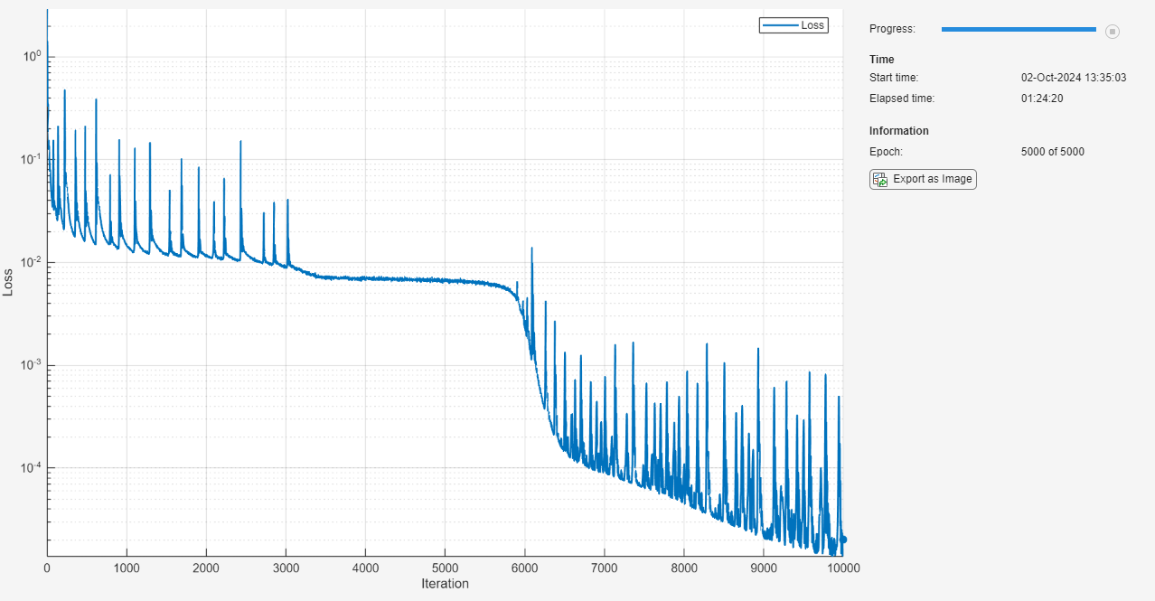
Monitor the training using a training progress monitor. Initialize a monitor that monitors the loss using the trainingProgressMonitor function. Monitor the loss using a log-scale plot. Because the timer starts when you create the monitor object, make sure that you create the object close to the training loop.

numObservations = size(XYTrain,1);
numIterationsPerEpoch = floor(numObservations / miniBatchSize);
numIterations = numEpochs * numIterationsPerEpoch;

monitor = trainingProgressMonitor( ...
    Metrics="Loss", ...
    Info="Epoch", ...
    XLabel="Iteration");
yscale(monitor,"Loss","log")

Train the model using a custom training loop.

For each epoch, shuffle the mini-batch queue and loop over mini-batches of training data. At the end of each epoch, update the training progress monitor and update the learning rate.

For each mini-batch:

• Evaluate the model loss and gradients using the dlfeval function with the accelerated model loss function.

• Update the neural network learnable parameters using the adamupdate function.

while epoch < numEpochs && ~monitor.Stop
    epoch = epoch + 1;

    shuffle(mbq);

    while hasdata(mbq) && ~monitor.Stop
        iteration = iteration + 1;

        [XY,U] = next(mbq);

        [loss,gradients] = dlfeval(lossFcn,net,XY,U,XYBoundaryTrain,UBoundaryTrain);

        [net,averageGrad,averageSqGrad] = adamupdate(net,gradients,averageGrad, ...
            averageSqGrad,iteration,learningRate);
    end

    learningRate = initialLearnRate / (1 + learnRateDecay*iteration);

    recordMetrics(monitor,iteration,Loss=loss);
    updateInfo(monitor,Epoch=epoch + " of " + numEpochs);
    monitor.Progress = 100 * iteration/numIterations;
end

Visualize Neural Network Predictions

Make predictions with the neural network using the training data.

[U,C] = predict(net,XYTrain);

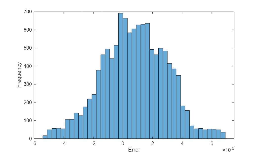
Visualize the error between the predictions and the targets.

figure
err = U - UTrain;
histogram(err)
xlabel("Error")
ylabel("Frequency")

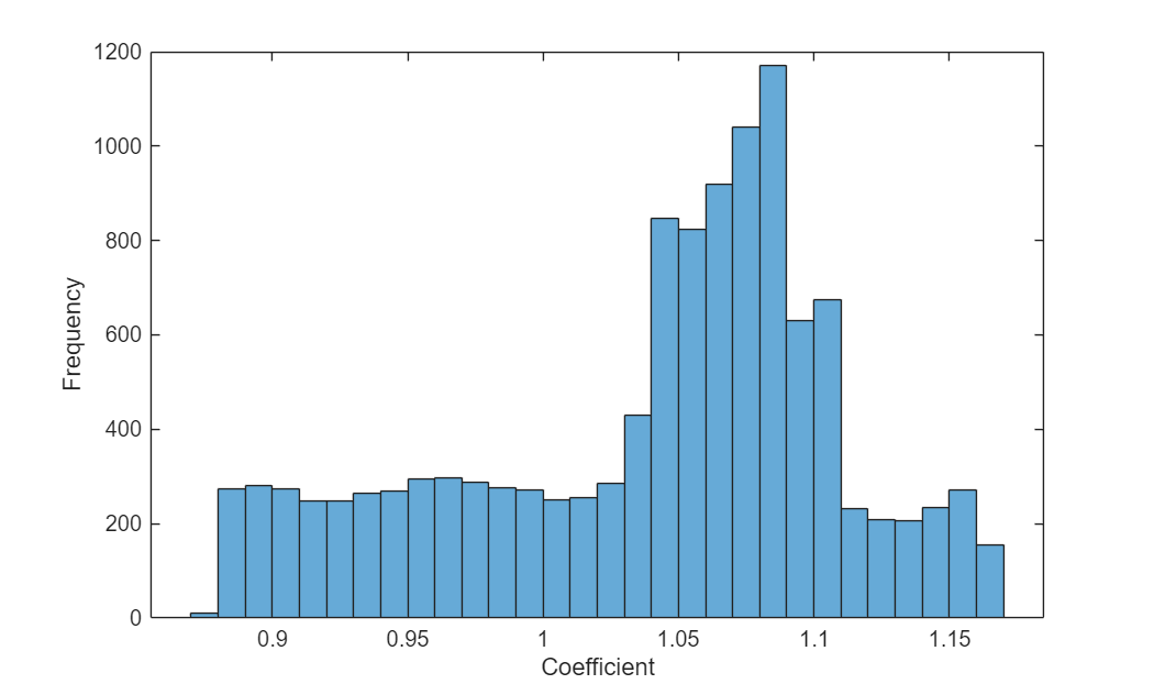
Visualize the distribution of the predicted coefficients.

figure
histogram(C)
xlabel("Coefficient")
ylabel("Frequency")

References

1. Raissi, Maziar, Paris Perdikaris, and George Em Karniadakis. "Physics Informed Deep Learning (Part I): Data-Driven Solutions of Nonlinear Partial Differential Equations." arXiv, November 28, 2017. https://doi.org/10.48550/arXiv.1711.10561

2. Guo, Yanan, Xiaoqun Cao, Junqiang Song, Hongze Leng, and Kecheng Peng. "An Efficient Framework for Solving Forward and Inverse Problems of Nonlinear Partial Differential Equations via Enhanced Physics-Informed Neural Network Based on Adaptive Learning." Physics of Fluids 35, no. 10 (October 1, 2023): 106603. https://doi.org/10.1063/5.0168390