Estimate Multiplicative ARIMA Model Using Econometric Modeler App

This example uses the Box-Jenkins method [1] to determine a multiplicative seasonal ARIMA (SARIMA) model for a univariate series by using the Econometric Modeler app. Specifically, the example shows this procedure:

1. Visually determine whether the series has an exponential trend, and then remove the trend if one is present.

   The remaining steps determine the structure of the conditional mean model to fit to the series without the exponential trend.

2. Visually determine whether the transformed series has seasonal integration, and then remove the seasonal integration, if it is present, by taking the seasonal difference. Record the degrees of seasonal integration removed.

3. Determine whether the transformed series has a unit root by conducting a statistical test, and then apply the first difference to the series to stabilize it, if a unit root is present. Record whether a unit root exists.

4. Determine the nonseasonal AR and MA degrees of the conditional mean model for the stationary series by inspecting correlograms of the stabilized series. Record the polynomial degrees.

5. Use the results of steps 2 through 4 to create and estimate a conditional mean model for the nonstationary series with the exponential trend removed.

The data set Data_Airline.mat contains monthly counts of airline passengers.

Import Data into Econometric Modeler

Download the Data_Airline.mat MAT-file into your current folder, and then load it into the workspace.

fldr = pwd;
openExample("Data_Airline.mat",workDir=fldr);
load(fullfile(fldr,"Data_Airline.mat"))

To change the folder to which to download the data set, set fldr to its absolute path.

At the command line, open the Econometric Modeler app.

econometricModeler

Alternatively, open the app from the apps gallery (see Econometric Modeler).

Import DataTimeTable into the app:

1. On the Modeler tab, in the Import section, click the Import button .

2. In the Import Data dialog box, select the check box for the DataTimeTable variable.

3. Click Import.

The variable PSSG appears in the Time Series pane, its value appears in the Preview pane, and its time series plot appears in the Plot(PSSG) figure window.

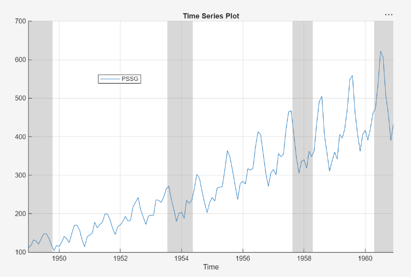
The series exhibits a seasonal trend, serial correlation, and possible exponential growth. For an interactive analysis of serial correlation, see Detect Serial Correlation Using Econometric Modeler App.

Stabilize Series

To properly determine the lag operator polynomial orders for the conditional mean model, correlograms require a stationary series.

Address the exponential trend by applying the log transform to PSSG.

1. In the Time Series pane, select PSSG.

2. On the Modeler tab, in the Transforms section, click Log.

The transformed variable PSSG_Log appears in the Time Series pane, its value appears in the Preview pane, and its time series plot appears in the Plot(PSSG_Log) figure window.

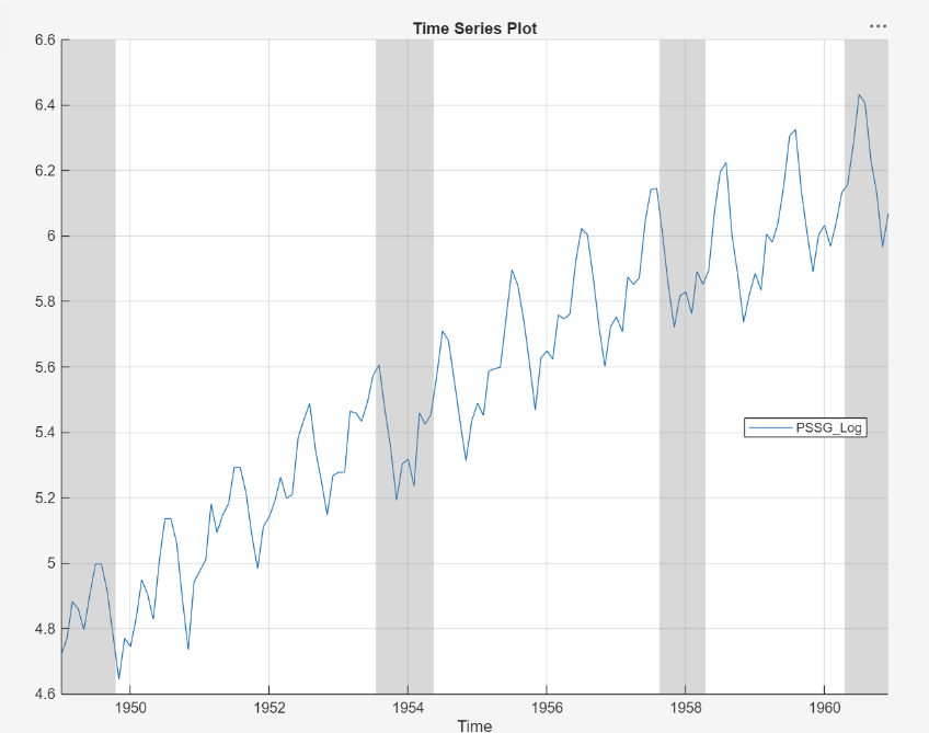
The exponential growth appears to be removed from the series.

The rest of the example determines the parameters of conditional mean model for the series PSSG_Log by several visual and statistical diagnoses and transformations.

Address the seasonal trend by applying the 12th order seasonal difference. With PSSG_Log selected in the Time Series pane, on the Modeler tab, in the Transforms section, set Seasonal to 12. Then, click Seasonal.

The transformed variable PSSG_Log_SDiff appears in the Time Series pane, and its time series plot appears in the Plot(PSSG_Log_SDiff) figure window.

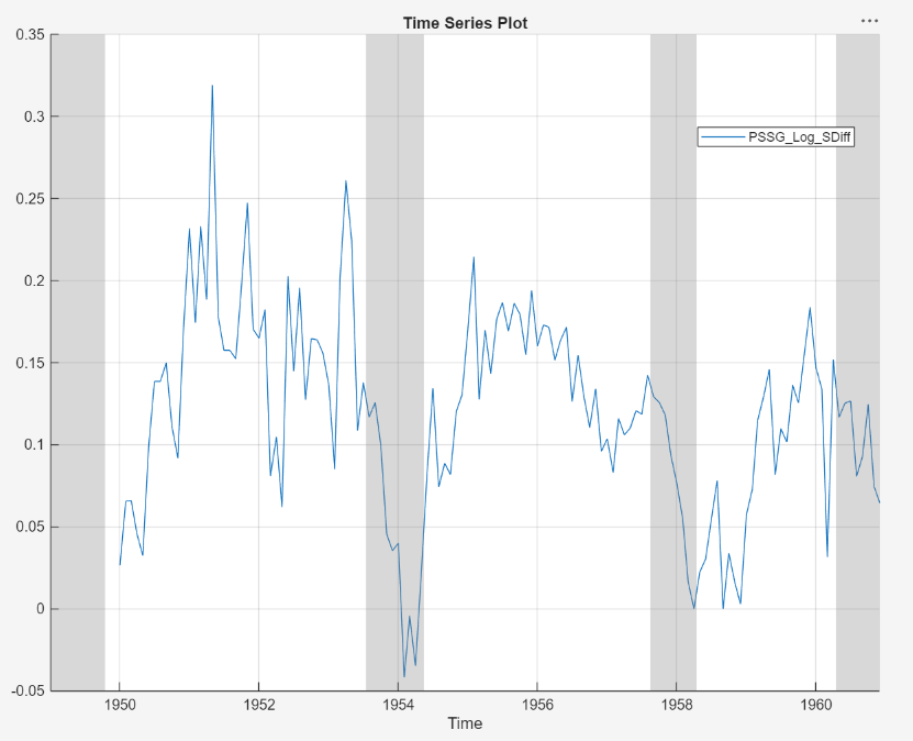
The transformed series appears to have a unit root.

Test the null hypothesis that PSSG_Log_SDiff has a unit root by using the Augmented Dickey-Fuller test. Specify that the alternative is an AR(0) model, then test again specifying an AR(1) model. Adjust the significance level to 0.025 to maintain a total significance level of 0.05.

1. With PSSG_Log_SDiff selected in the Time Series pane, on the Modeler tab, in the Tests section, click Add Test > Augmented Dickey-Fuller Test.

2. On the ADF tab, in the Settings section, set Significance Level to 0.025.

3. In the Tests section, click Run Test.

4. In the Settings section, set Number of Lags to 1.

5. In the Tests section, click Run Test.

The test results appear in the Results table of the ADF(PSSG_Log_SDiff) document.

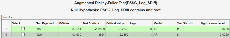
Both tests fail to reject the null hypothesis that the series is a unit root process.

Address the unit root by applying the first difference to PSSG_Log_SDiff. With PSSG_Log_SDiff selected in the Time Series pane, click the Modeler tab. Then, in the Transforms section, click Difference.

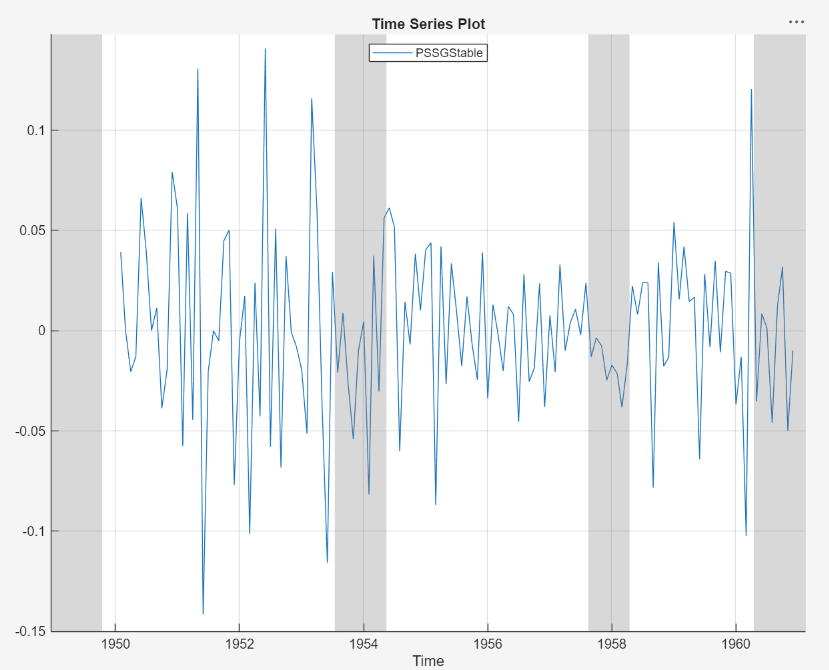
The transformed variable PSSG_Log_SDiff_Diff appears in the Time Series pane, and its time series plot appears in the Plot(PSSG_Log_SDiff_Diff) figure window.

In the Time Series pane, rename the PSSG_Log_SDiff_Diff variable by clicking it twice to select its name and entering PSSGStable.

The app updates the names of all documents associated with the transformed series.

Identify Model for Series

Determine the lag structure for a conditional mean model of the series by plotting the sample autocorrelation function (ACF) and partial autocorrelation function (PACF) of the stabilized series.

1. With PSSGStable selected in the Time Series pane, click the Plots tab, then click ACF.

2. Show the first 50 lags of the ACF. On the ACF tab, set Number of Lags to 50.

3. Click the Plots tab, then click PACF.

4. Show the first 50 lags of the PACF. On the PACF tab, set Number of Lags to 50.

5. Drag the ACF(PSSGStable) figure window above the PACF(PSSGStable) figure window.

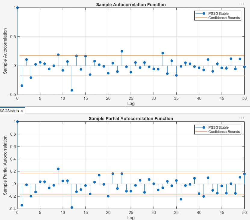
According to [1], the autocorrelations in the ACF and PACF, the results in previous steps, and the balance of model parsimony with complexity, suggest that the following SARIMA(0,1,1)×(0,1,1)₁₂ model is appropriate for the nonstationary series with the exponential trend removed PSSG_Log.

$$(1-L)\left(1-L^{12}\right)y_t=\left(1+{\theta }_{1}L\right)\left(1+{\Theta }_{12}{L}^{12}\right){\epsilon }_t.$$

Close all figure windows.

Specify and Estimate SARIMA Model

Specify the SARIMA(0,1,1)×(0,1,1)₁₂ model.

1. In the Time Series pane, select the PSSG_Log time series.

2. On the Modeler tab, in the Models section, click the arrow > SARIMA.

3. In the SARIMA Model Parameters dialog box, on the Lag Order tab:

   • Nonseasonal section

     1. Set Autoregressive Order (p) to 0.

     2. Clear the Include Constant Term check box.

   • Seasonal section

     1. Set Autoregressive Order (p_s) to 0.

     2. The Seasonality (s) parameter is 12 by default; this setting indicates monthly periodicity.

   

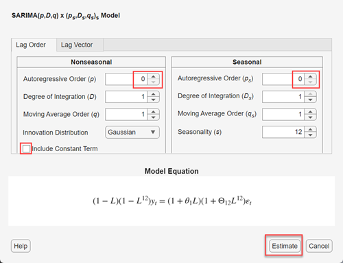
4. Click Estimate.

The model variable SARIMA_PSSG_Log appears in the Models pane, its value appears in the Preview pane, and its estimation summary appears in the Fit(SARIMA_PSSG_Log) document.

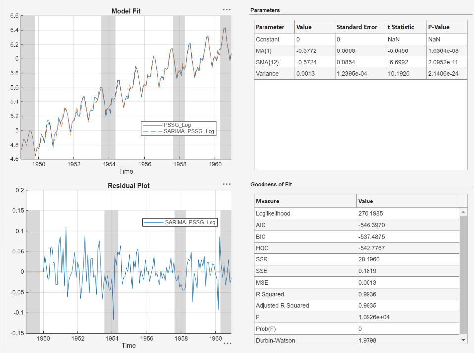
The results include:

• Model Fit — A time series plot of PSSG_Log and the fitted values from SARIMA_PSSG_Log.

• Residual Plot — A time series plot of the residuals of SARIMA_PSSG_Log.

• Parameters — A table of estimated parameters of SARIMA_PSSG_Log. Because the constant term was held fixed to 0 during estimation, its value and standard error are 0.

• Goodness of Fit — Model fit statistics, such as the AIC and BIC fit statistics of SARIMA_PSSGLog.

References

[1] Box, George E. P., Gwilym M. Jenkins, and Gregory C. Reinsel. Time Series Analysis: Forecasting and Control. 3rd ed. Englewood Cliffs, NJ: Prentice Hall, 1994.