Simulate Paths of Threshold-Switching Dynamic Regression Models

The example shows how to generate random response, innovations, and state paths of various threshold-switching dynamic regression models by using the simulate function.

Simulate Model Containing Exogenous Threshold Variable

Consider the Canadian inflation and interest rates data set Data_Canada.mat, which contains the CPI-based inflation rate series INF_C, among other series. Load the data set and extract INF_C.

load Data_Canada
INF_C = DataTable.INF_C;
numObs = length(INF_C);

Model simulation requires a fully specified model. Create a univariate, three-state, mean-variance-switching, smooth threshold autoregressive (STAR) model for an arbitrary response variable in the data set with the following characteristics:

• The threshold variable is INF_C.

• The threshold transitions are at mid-levels 2 and 8, the transition function is logistic, the transition rate from state 1 to 2 is 3.5, and the rate from state 2 to 3 is 1.5.

• The state 1 submodel is ${\mathit{y}}_{1,\mathit{t}}=-5+{\epsilon }_{1,\mathit{t}}$, where ${\epsilon }_{1,\mathit{t}}\sim {\rm N}\left(0,0.1\right)$.

• The state 2 submodel is ${\mathit{y}}_{2,\mathit{t}}={\epsilon }_{2,\mathit{t}}$, where ${\epsilon }_{2,\mathit{t}}\sim {\rm N}\left(0,0.3\right)$.

• The state 3 submodel is ${\mathit{y}}_{3,\mathit{t}}=5+{\epsilon }_{3,\mathit{t}}$, where ${\epsilon }_{3,\mathit{t}}\sim {\rm N}\left(0,0.5\right)$.

ttL = threshold([2 8],Type="logistic",Rates=[3.5 1.5]);

mdl1 = arima(Constant=-5,Variance=0.1);
mdl2 = arima(Constant=0,Variance=0.3);
mdl3 = arima(Constant=5,Variance=0.5);

Mdl1 = tsVAR(ttL,[mdl1 mdl2 mdl3],SeriesNames="y")

Mdl1 = 
  tsVAR with properties:

         Switch: [1x1 threshold]
      Submodels: [3x1 varm]
      NumStates: 3
      NumSeries: 1
     StateNames: ["1"    "2"    "3"]
    SeriesNames: "y"
     Covariance: []

Mdl1 is a tsVAR object representing the STAR model. The model is agnostic of the threshold variable at this point. It is aware only of the characteristics of the threshold transitions.

Generate 10 sample paths of the STAR model. To simulate observations, the model requires threshold variable data to trigger state switching. Specify INF_C as the exogenous threshold variable data.

rng(0) % For reproducibility
y = simulate(Mdl1,numObs,NumPaths=10,Type="exogenous",Z=INF_C);

y is a numObs-by-10 numeric matrix of independent, simulated paths. The rows correspond to periods in the data and the columns correspond to the generated paths.

In the same figure, plot the threshold transitions and the threshold data in the same plot, and plot the simulated responses.

figure
tiledlayout(2,1)
nexttile
ttplot(ttL,'Data',INF_C)
title('Threshold Variable')
colorbar('off')
nexttile
plot(y)
title("Simulations")
grid on
axis tight

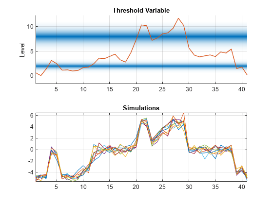
The submodels have conditional means –5, 0, and 5 with innovations variances 0.1, 0.2, and 0.3. The response y switches between submodels according to the value of the threshold variable INF_C. Because Mdl1.Covariance is empty, simulate generates innovations by using the submodel covariances. Regime mixing is evident near transitions, for example, near observations 10 and 25.

Simulate Models Containing Endogenous Threshold Variable

Models can be self-exciting, where simulations use an endogenous, lagged component of the response as a threshold variable.

Create a threshold-switching model with the following characteristics:

• The threshold transitions are at mid-levels 2 and 8, and the transition function is discrete.

• The state 1 submodel is ${\mathit{y}}_{1,\mathit{t}}=\left[\begin{array}{c}0\\ 0\end{array}\right]+{\epsilon }_{\mathit{t}}$.

• The state 2 submodel is ${\mathit{y}}_{2,\mathit{t}}=\left[\begin{array}{c}-5\\ 5\end{array}\right]+{\epsilon }_{\mathit{t}}$.

• The state 3 submodel is ${\mathit{y}}_{3,\mathit{t}}=\left[\begin{array}{c}-10\\ 10\end{array}\right]+{\epsilon }_{\mathit{t}}$.

• The model-wide innovation variable ${\epsilon }_{\mathit{t}}\sim \mathit{N}\left(\left[\begin{array}{c}0\\ 0\end{array}\right],\left[\begin{array}{cc}5& 0\\ 0& 5\end{array}\right]\right)$.

ttD = threshold([2 8]);

mdl1 = varm(Constant=[0; 0]);
mdl2 = varm(Constant=[-5; 5]);
mdl3 = varm(Constant=[-10; 10]);

Sigma = 5*eye(2);
SimMdl2 = tsVAR(ttD,[mdl1 mdl2 mdl3],Covariance=Sigma);

Simulate 30 periods of the self-exciting TAR (SETAR) model. Specify that the threshold variable is the second response variable with a delay of 5 periods. Return simulated responses, innovations, and states.

rng(0)
[Y,E,SP] = simulate(SimMdl2,30,Type="endogenous",Index=1,Delay=5); 

figure
tiledlayout(4,1)
nexttile
ttplot(ttD,Data=Y(:,1))
title('Threshold Variable')

nexttile
plot(Y)
title("Simulation")
legend(["Y1" "Y2"])
grid on

nexttile
plot(E)
title("Innovations")
legend(["E1" "E2"])
grid on

nexttile
stem(SP)
title("State Path")

The simulation starts in state 1, below the first threshold level, where both components of the response have a conditional mean of 0. At the 5th observation, a large innovation drives the first component of the response Y1, which is the self-exciting threshold variable, over the second threshold level and into state 3. Because the delay is 5, a switch to state 3 occurs at the 10th observation, where the two components of the response center on distinct conditional means of -10 and 10. The pattern is repeated at the 20th and 25th observations, where a switch from state 1 to state 2 causes a delayed response to components centered on conditional means of -5 and 5.

Include negative autoregression to the submodel in the first state to generate paths with more level crossings and subsequent state changes.

mdl1.AR = {[-0.6 0; 0 0]};

SimMdl2 = tsVAR(ttD,[mdl1 mdl2 mdl3],Covariance=Sigma);

Y = simulate(SimMdl2,30,Type="endogenous",Index=1,Delay=5);

figure
tiledlayout(2,1)
nexttile
ttplot(ttD,Data=Y(:,1))
title("Threshold Variable")

nexttile
plot(Y)
title("Simulation")
legend(["Y1" "Y2"])
grid on

Include a regression component to the submodel in the first state to change the dynamics to be more cyclic.

mdl1.Beta = [1 1; -1 -1];
X = 5*rand(30,2);

SimMdl3 = tsVAR(ttD,[mdl1 mdl2 mdl3],Covariance=Sigma);

Y = simulate(SimMdl3,30,Type="endogenous",Index=1,Delay=5,X=X);

figure
tiledlayout(2,1)
nexttile
ttplot(ttD,Data=Y(:,1))
title("Threshold Variable")

nexttile
plot(Y)
title("Simulation")
legend(["Y1" "Y2"])
grid on

Change the transition function to a smooth logistic distribution to produce a model with mixed dynamics and a damped response.

ttL2 = threshold([2 8],Type="logistic",Rates=[0.2 0.3]);
SimMdl4 = tsVAR(ttL2,[mdl1 mdl2 mdl3],Covariance=Sigma);

YS = simulate(SimMdl4,30,Type="endogenous",Index=1,Delay=5,X=X);

figure
x = 1:30;
plot(x,Y(x,1),"r-",x,YS(x,1),"b--")
title("Simulations")
legend(["TAR" "STAR"])
grid on

The plot shows the self-exciting component of the response Y1 in the two models. The logistic transitions in the STAR model result in mixing of submodel responses. When submodels of lower absolute conditional means mix with those of higher absolute conditional means, the result is mean reversion toward 0.