Risk Parity or Budgeting with Constraints
This example shows how to solve risk parity or budgeting problems with constraints using estimateCustomObjectivePortfolio.
Risk parity is a portfolio allocation strategy that focuses on the allocation of risk to define the weights of a portfolio. You construct the risk parity portfolio, or equal risk contribution portfolio, by ensuring that all assets in a portfolio have the same risk contribution to the overall portfolio risk. The generalization of this problem is the risk budgeting portfolio in which you set the risk contribution of each asset to the overall portfolio risk. In other words, instead of all assets contributing equally to the risk of the portfolio, the assets' risk contribution must match a target risk budget.
In Risk Budgeting Portfolio, the example describes some advantages of risk parity or budgeting portfolios. It shows how to use riskBudgetingPortfolio to solve long-only, fully invested risk parity or budgeting problems. When the only constraints of the risk budgeting problem enforce nonnegative weights that sum to 1, the risk budgeting problem is a feasibility problem. In other words, the solution to the problem is the one that exactly matches the target risk budget and it is unique. Therefore, there is no need for an objective function. The riskBudgetingPortfolio function is optimized to solve this specific type of problems.
When you add more constraints to the risk parity problem, you must find the weight allocation that satisfies the extra constraints while trying to match the target risk budget as much as possible. The next section explains how.
Define Problem
Start by defining the problem data.
% Assets variance
vol = [0.1;0.15;0.2;0.3];
% Assets correlation
rho = [1.00  0.50  0.50  0.50;
       0.50  1.00  0.50  0.50;
       0.50  0.50  1.00  0.75;
       0.50  0.50  0.75  1.00];
% Assets covariance matrix
Sigma = corr2cov(vol,rho);
% Risk budget
budget = [0.3;0.3;0.195;0.205];
Obtain the long-only, fully invested risk budgeting portfolio to use as benchmark.
% Long-only fully invested risk budgeting portfolio
w_simple = riskBudgetingPortfolio(Sigma,budget);
% Compute the risk contribution of the weight allocation
RC_simple = portfolioRiskContribution(w_simple,Sigma);
% Table with weights and risk contributions
T_simple = table(w_simple,RC_simple,budget, ...
    VariableNames={'RB Portfolio','RB Contribution','Budget'})
T_simple=4×3 table
    RB Portfolio    RB Contribution    Budget
    ____________    _______________    ______

      0.45053              0.3           0.3
      0.30035              0.3           0.3
      0.14668            0.195         0.195
      0.10244            0.205         0.205
As desired, the risk contribution of the risk budgeting portfolio matches the budget.
Add Constraints to Risk Parity or Budgeting Portfolio
When you add constraints, other than the long-only, fully invested constraints, to the risk parity formulation, you must find the portfolio allocation that satisfies all the constraints and minimizes the deviation from the target risk budget.
The percent risk contribution of asset is defined as
,
and the goal is to find the portfolio that minimizes the deviation of to , the target risk budget of asset . For risk parity problems, , where is the number of assets.
A common way to measure deviation is to use a norm. In this example, use the 2-norm. The risk parity or budgeting problem with constraints results in
where represents the feasible set that is defined by the desired constraints. The objective function is the sum of squares of the deviation of the risk contributions from the target. Notice that the objective function is nonconvex.
Next, introduce the constraint , which means that no more than 30% of the capital can be invested in each asset.
% Define the Portfolio object
p = Portfolio(AssetCovar=Sigma);
% Set bound constraints
p = setBounds(p,0,0.3);
% Set budget constraint
p = setBudget(p,1,1);
Create a function handle for the nonconvex objective
.
% Define objective function
objFun = @(w) sum(((w.*(Sigma*w))/(w'*Sigma*w) - budget).^2);
Solve the problem using estimateCustomObjectivePortfolio and riskBudgetingPortfolio.
% Risk budgeting portfolio with extra constraints
w_extra = estimateCustomObjectivePortfolio(p,objFun);
% Risk contribution
RC_extra = portfolioRiskContribution(w_extra,Sigma);
% Table with weights and risk contributions
T_extra = table(w_extra,RC_extra,budget, ...
    VariableNames={'RB Portfolio','RB Contribution','Budget'})
T_extra=4×3 table
    RB Portfolio    RB Contribution    Budget
    ____________    _______________    ______

          0.3           0.15505          0.3
          0.3           0.24998          0.3
       0.2465           0.30862        0.195
       0.1535           0.28635        0.205
Now that you have added additional constraints, the risk contribution of the resulting portfolio does not match the budget. Yet, the solution to the problem is minimizing the deviation of the risk contribution to the target risk budget. Because the risk budgeting portfolio without the extra constraints assigns weights larger than 30% to the first and second assets, the solution to the problem that minimizes the deviation assigns as much as possible to the first and second assets and distributes the rest to the other assets.
As explained in Role of Convexity in Portfolio Problems, because the objective function is nonconvex, this formulation cannot be solved by the Portfolio object solvers if you add cardinality constraints or conditional bounds to the problem.
Compare Risk Parity and Mean-Variance Portfolios
You can examine the difference in the allocation between the traditional minimum variance portfolio and the risk parity portfolio.
First compute the minimum variance portfolio. The traditional mean-variance framework requires the assets mean return to be defined before you compute any of the portfolios on the efficient frontier.
% Define assets mean
p.AssetMean = [0.1; 0.1; 0.15; 0.2];
% Minimum variance portfolio
wMinVar = estimateFrontierLimits(p,'min');
To compute the risk parity portfolio, make sure all assets contribute equally to the risk. Set and update the objective function.
% Update budget
budget = 1/p.NumAssets*ones(p.NumAssets,1);
% Update objective
objFun = @(w) sum(((w.*(Sigma*w))/(w'*Sigma*w) - budget).^2);
Solve the risk parity problem using estimateCustomObjectivePortfolio.
% Risk parity portfolio with extra constraints
wRP = estimateCustomObjectivePortfolio(p,objFun);
Compare the weight allocation concentrations.
% Plot pie charts
tiledlayout(1,2);
% Minimum variance portfolio
nexttile
pie(wMinVar)
title('Minimum Variance Portfolio',Position=[0,1.5]);
% Risk parity portfolio
nexttile
pie(wRP)
title('Risk Parity Portfolio',Position=[0,1.5]);

% Add legend
lgd = legend({'1','2','3','4'});
lgd.Layout.Tile = 'east';
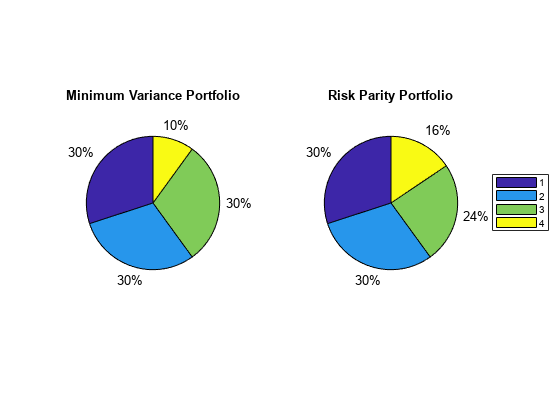
The portfolio allocation of the minimum variance portfolio sets all assets with the smallest risk to their maximum (30%). On the other hand, the risk parity allocation sets only the first two assets to 30% and the last two are more balanced. This result is a simple example of how the risk parity allocation helps to diversify a portfolio.
See Also
estimatePortSharpeRatio | estimateFrontier | estimateFrontierByReturn | estimateFrontierByRisk | estimateCustomObjectivePortfolio
Topics
- Diversify Portfolios Using Custom Objective
- Portfolio Optimization Using Social Performance Measure
- Diversify Portfolios Using Custom Objective
- Portfolio Optimization Against a Benchmark
- Solve Tracking Error Portfolio Problems
- Solve Problem for Minimum Tracking Error with Net Return Constraint
- Solve Robust Portfolio Maximum Return Problem with Ellipsoidal Uncertainty
- Solver Guidelines for Custom Objective Problems Using Portfolio Objects