Automated Fixed-Point Conversion
License Requirements
Fixed-point conversion requires the following licenses:
Fixed-Point Designer™
MATLAB® Coder™
Automated Fixed-Point Conversion Capabilities
You can convert floating-point MATLAB code to fixed-point code using the Fixed-Point Conversion step in the HDL Workflow Advisor for your HDL Coder™ projects. You can choose to propose data types based on simulation range data, derived (also known as static) range data, or both.
You can manually enter static ranges. These manually-entered ranges take precedence over simulation ranges and the tool uses them when proposing data types. In addition, you can modify and lock the proposed type so that the tool cannot change it. For more information, see Locking Proposed Data Types.
For a list of supported MATLAB features and functions, see MATLAB Language Features Supported for Automated Fixed-Point Conversion.
During fixed-point conversion, you can:
Verify that your test files cover the full intended operating range of your algorithm using code coverage results.
Propose fraction lengths based on default word lengths.
Propose word lengths based on default fraction lengths.
Optimize whole numbers.
Specify safety margins for simulation min/max data.
Validate that you can build your project with the proposed data types.
Test numerics by running the test bench with the fixed-point types applied.
View a histogram of bits used by each variable.
Detect overflows.
Code Coverage
By default, the Fixed-Point Conversion tool shows code coverage results. Your test files must exercise the algorithm over its full operating range so that the simulation ranges are accurate. The quality of the proposed fixed-point data types depends on how well the test files cover the operating range of the algorithm with the accuracy that you want. Reviewing code coverage results helps you verify that your test files are exercising the algorithm adequately. If the code coverage is inadequate, modify the test files or add more test files to increase coverage. If you simulate multiple test files in one run, the tool displays cumulative coverage. However, if you specify multiple test files but run them one at a time, the tool displays the coverage of the file that ran last.
The tool displays a color-coded coverage bar to the left of the code.

This table describes the color coding.
| Coverage Bar Color | Indicates |
|---|---|
| Green | One of the following situations:
Different shades of green indicate different ranges of line execution counts. The darkest shade of green indicates the highest range. |
| Orange | The entry-point function executes multiple times, but the code executes one time. |
| Red | Code does not execute. |
When you pause over the coverage bar, the color highlighting extends over the code. For each section of code, the app displays the number of times that section executes.
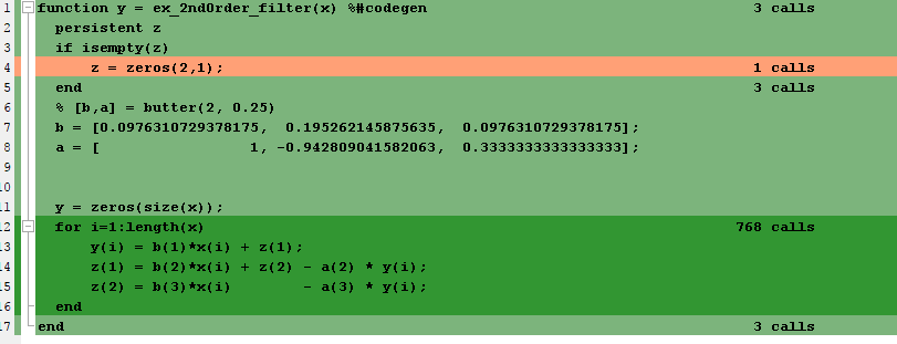
To verify that your test files are testing your algorithm over the intended operating range, review the code coverage results.
| Coverage Bar Color | Action |
|---|---|
| Green | If you expect sections of code to execute more frequently than the coverage shows, either modify the MATLAB code or the test files. |
| Orange | This behavior is expected for initialization code, for example, the initialization of persistent variables. If you expect the code to execute more than one time, either modify the MATLAB code or the test files. |
| Red | If the code that does not execute is an error condition, this behavior is acceptable. If you expect the code to execute, either modify the MATLAB code or the test files. If the code is written conservatively and has upper and lower boundary limits, and you cannot modify the test files to reach this code, add static minimum and maximum values. See Computing Derived Ranges. |
Code coverage is on by default. Turn it off only after you have verified that you have adequate test file coverage. Turning off code coverage can speed up simulation. To turn off code coverage, in the Fixed-Point Conversion tool:
Click Run Simulation.
Clear
Show code coverage.
Proposing Data Types
In the Define Input Types step, you specify a test bench that calls the MATLAB function. The tool runs the test file to analyze the code and infer the types for entry-point input arguments.

The Fixed-Point Conversion tool proposes fixed-point data types based on computed ranges and the word length or fraction length setting. The computed ranges are based on simulation range data, derived range data, or both. If you run a simulation and compute derived ranges, the conversion tool merges the simulation and derived ranges.
Note
You cannot propose data types based on derived ranges for MATLAB classes.
You can manually enter static ranges. These manually-entered ranges take precedence over simulation ranges and the tool uses them when proposing data types. If you analyze ranges using derived range analysis alone, you must enter static ranges. In addition, you can modify and lock the proposed type so that the tool cannot change it. For more information, see Locking Proposed Data Types.
Running a Simulation
When you open the Fixed-Point Conversion tool, the tool generates an instrumented MEX function for your MATLAB design. If the build completes without errors, the tool displays compiled information (type, size, complexity) for functions and variables in your code. To navigate to local functions, click the Functions tab. If build errors occur, the tool provides error messages that link to the line of code that caused the build issues. You must address these errors before running a simulation. Use the link to navigate to the offending line of code in the MATLAB editor and modify the code to fix the issue.
If your code uses functions that are not supported for fixed-point conversion, the tool
displays them on the Function Replacements tab. See Function Replacements. You can also use coder.float2fixed.skip to omit these functions from fixed-point conversion.
Before running a simulation, specify the test bench that you want to run. When you run a simulation, the tool runs the test bench, calling the instrumented MEX function. If you modify the MATLAB design code, the tool automatically generates an updated MEX function before running the test bench.
If the test bench runs successfully, the simulation minimum and maximum values and the proposed types are displayed on the Variables tab. If you manually enter static ranges for a variable, the manually-entered ranges take precedence over the simulation ranges. If you manually modify the proposed types by typing or using the histogram, the data types are locked so that the tool cannot modify them.
If the test bench fails, the errors are displayed on the Simulation Output tab.
The test bench should exercise your algorithm over its full operating range. The quality of the proposed fixed-point data types depends on how well the test bench covers the operating range of the algorithm with the desired accuracy.
Optionally, you can select to log data for histograms. After running a simulation, you can view the histogram for each variable. For more information, see Histogram.
Computing Derived Ranges
The advantage of proposing data types based on derived ranges is that you do not have to provide test files that exercise your algorithm over its full operating range. Running such test files often takes a very long time.
To compute derived ranges and propose data types based on these ranges, provide static minimum and maximum values or proposed data types for all input variables. To improve the analysis, enter as much static range information as possible for other variables. You can manually enter ranges or promote simulation ranges to use as static ranges. Manually-entered static ranges always take precedence over simulation ranges.
If you know what data type your hardware target uses, set the proposed data types to match this type. Manually-entered data types are locked so that the tool cannot modify them. The tool uses these data types to calculate the input minimum and maximum values and to derive ranges for other variables. For more information, see Locking Proposed Data Types.
When you select Compute Derived Ranges,
the tool runs a derived range analysis to compute static ranges for
variables in your MATLAB algorithm. When the analysis is complete,
the static ranges are displayed on the Variables tab.
If the run produces +/-Inf derived ranges, consider
defining ranges for all persistent
variables.
Optionally, you can select Quick derived range analysis. With this option, the conversion tool performs faster static analysis. The computed ranges might be larger than necessary. Select this option in cases where the static analysis takes more time than you can afford.
If the derived range analysis for your project is taking a long time, you can optionally set a timeout. The tool aborts the analysis when the timeout is reached.
Locking Proposed Data Types
You can lock proposed data types against changes by the Fixed-Point Conversion tool using one of the following methods:
Manually setting a proposed data type in the Fixed-Point Conversion tool.
Right-clicking a type proposed by the tool and selecting
Lock
computed value
.
The tool displays locked data types in bold so that they are easy to identify. You can unlock a type using one of the following methods:
Manually overwriting it.
Right-clicking it and selecting
Undo
changes
. This action unlocks only the selected type.Right-clicking and selecting
Undo changes
for all variables
. This action unlocks all locked proposed types.
Viewing Functions
You can view a list of functions in your project on the Navigation pane. This list also includes function specializations and class methods. When you select a function from the list, the MATLAB code for that function or class method is displayed in the Fixed-Point Conversion tool code window.
After conversion, the left pane also displays a list of output
files including the fixed-point version of the original algorithm.
If your function is not specialized, the conversion retains the original
function name in the fixed-point filename and appends the fixed-point
suffix. For example, the fixed-point version of fun_with_matlab.m is fun_with_matlab_fixpt.m.
Viewing Variables
The Variables tab provides the following information for each variable in the function selected in the Navigation pane:
Type — The original data type of the variable in the MATLAB algorithm.
Sim Min and Sim Max — The minimum and maximum values assigned to the variable during simulation.
You can edit the simulation minimum and maximum values. Edited fields are shown in bold. Editing these fields does not trigger static range analysis, but the tool uses the edited values in subsequent analyses. You can revert to the types proposed by the tool.
Static Min and Static Max — The static minimum and maximum values.
To compute derived ranges and propose data types based on these ranges, provide static minimum and maximum values for all input variables. To improve the analysis, enter as much static range information as possible for other variables.
When you compute derived ranges, the Fixed-Point Conversion tool runs a static analysis to compute static ranges for variables in your code. When the analysis is complete, the static ranges are displayed. You can edit the computed results. Edited fields are shown in bold. Editing these fields does not trigger static range analysis, but the tool uses the edited values in subsequent analyses. You can revert to the types proposed by the tool.
Whole Number — Whether all values assigned to the variable during simulation are integers.
The Fixed-Point Conversion tool determines whether a variable is always a whole number. You can modify this field. Edited fields are shown in bold. Editing these fields does not trigger static range analysis, but the tool uses the edited values in subsequent analyses. You can revert to the types proposed by the tool.
The proposed fixed-point data type for the specified word (or fraction) length. Proposed data types use the
numerictypenotation. For example,numerictype(1,16,12)denotes a signed fixed-point type with a word length of 16 and a fraction length of 12.numerictype(0,16,12)denotes an unsigned fixed-point type with a word length of 16 and a fraction length of 12.Because the tool does not apply data types to expressions, it does not display proposed types for them. Instead, it displays their original data types.
You can also view and edit variable information in the code pane by placing your cursor over a variable name.
You can use Ctrl+F to search for variables
in the MATLAB code and on the Variables tab.
The tool highlights occurrences in the code and displays only the
variable with the specified name on the Variables tab.
Viewing Information for MATLAB Classes
The tool displays:
Code for MATLAB classes and code coverage for class methods in the code window. Use the Function list in the Navigation bar to select which class or class method to view.
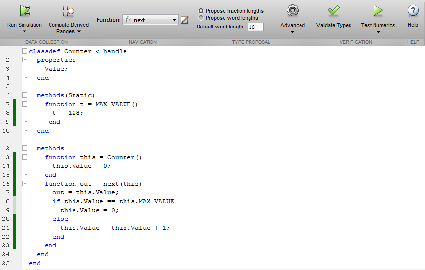
Information about MATLAB classes on the Variables tab.

Specializations
If a function is specialized, the tool lists each specialization
and numbers them sequentially. For example, consider a function, dut,
that calls subfunctions, foo and bar,
multiple times with different input types.
function y = dut(u, v)

tt1 = foo(u);
tt2 = foo([u v]);
tt3 = foo(complex(u,v));

ss1 = bar(u);
ss2 = bar([u v]);
ss3 = bar(complex(u,v));

y = (tt1 + ss1) + sum(tt2 + ss2) + real(tt3) + real(ss3);

end

function y = foo(u)
  y = u * 2;
end

function y = bar(u)
  y = u * 4;
end
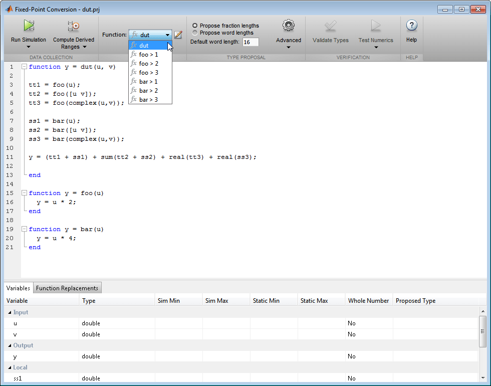
If you select a specialization, the app displays only the variables used by the specialization.
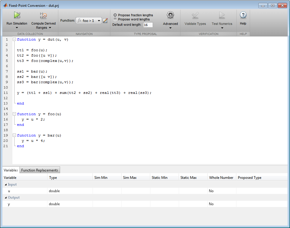
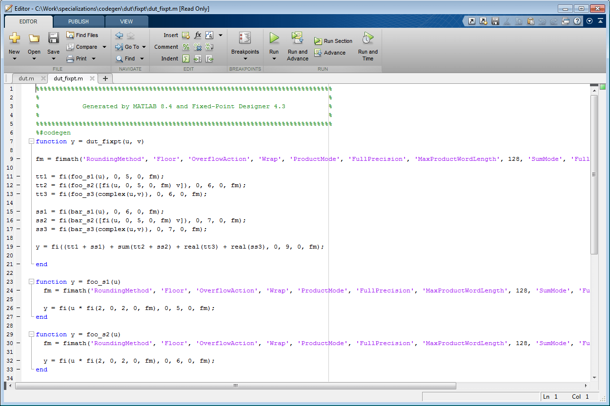
In the generated fixed-point code, the number of each fixed-point
specialization matches the number in the Source Code list which makes
it easy to trace between the floating-point and fixed-point versions
of your code. For example, the generated fixed-point function for foo
> 1 is named foo_s1.
Histogram
To log data for histograms, in the Fixed-Point Conversion window, click Run
Simulation and select Log data for histogram, and then
click the Run Simulation button.
After simulation, to view the histogram for a variable, on the Variables tab, click the Proposed Type field for that variable.
The histogram provides the range of the proposed data type and the percentage of simulation
values that the proposed data type covers. The bit weights are displayed along the
X-axis, and the percentage of occurrences along the
Y-axis. Each bin in the histogram corresponds to a bit in the binary
word. For example, this histogram displays the range for a variable of type
numerictype(1,16,14).
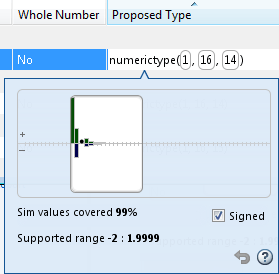
You can view the effect of changing the proposed data types by:
Dragging the edges of the bounding box in the histogram window to change the proposed data type.
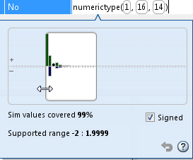
Selecting or clearing Signed.
To revert to the types proposed by the automatic conversion,
in the histogram window, click ![]() .
.
Function Replacements
If your MATLAB code uses functions that do not have fixed-point support, the tool lists these functions on the Function Replacements tab. You can choose to replace unsupported functions with a custom function replacement or with a lookup table.
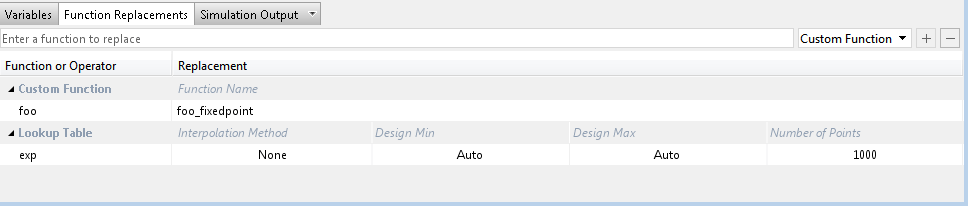
You can add and remove function replacements from this list. If you enter a function replacements for a function, the replacement function is used when you build the project. If you do not enter a replacement, the tool uses the type specified in the original MATLAB code for the function.
Note
Using this table, you can replace the names of the functions but you cannot replace argument patterns.
Alternatively, you can exclude functions from fixed-point conversion using
coder.float2fixed.skip. For example, you may want to exclude a function
from fixed-point conversion if you are using a custom function that already uses fixed-point
data types, or if you want to take advantage of native floating point support for HDL Code
generation. For more information, see coder.float2fixed.skip.
Validating Types
Selecting Validate Types validates the build using the proposed fixed-point data types. If the validation is successful, you are ready to test the numerical behavior of the fixed-point MATLAB algorithm.
If the errors or warnings occur during validation, they are displayed on the Type Validation Output tab. If errors or warning occur:
On the Variables tab, inspect the proposed types and manually modified types to verify that they are valid.
On the Function Replacements tab, verify that you have provided function replacements for unsupported functions.
Testing Numerics
After validating the proposed fixed-point data types, select Test Numerics to verify the behavior of the fixed-point MATLAB algorithm. By default, if you added a test bench to define inputs or run a simulation, the tool uses this test bench to test numerics. The tool compares the numerical behavior of the generated fixed-point MATLAB code with the original floating-point MATLAB code. If you select to log inputs and outputs for comparison plots, the tool generates an additional plot for each scalar output. This plot shows the floating-point and fixed-point results and the difference between them. For non-scalar outputs, only the error information is shown.
If the numerical results do not meet your desired accuracy after fixed-point simulation, modify fixed-point data type settings and repeat the type validation and numerical testing steps. You might have to iterate through these steps multiple times to achieve the desired results.
Detecting Overflows
When testing numerics, selecting Use scaled doubles to detect overflows enables overflow detection. When this option is selected, the conversion tool runs the simulation using scaled double versions of the proposed fixed-point types. Because scaled doubles store their data in double-precision floating-point, they carry out arithmetic in full range. They also retain their fixed-point settings, so they are able to report when a computation goes out of the range of the fixed-point type.
If the tool detects overflows, on its Overflow tab, it provides:
A list of variables and expressions that overflowed
Information on how much each variable overflowed
A link to the variables or expressions in the code window
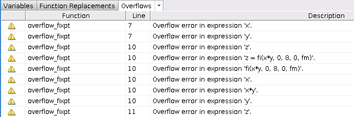
If your original algorithm uses scaled doubles, the tool also provides overflow information for these expressions.