psf

R2026b

Compute point spread function of optical system

Since R2026b

Syntax

psfr = psf(opsys)

psfr = psf(opsys,Name=Value)

Description

Add-On Required: This feature requires the Optical Design and Simulation Library for Image Processing Toolbox add-on.

psfr = psf(opsys) computes the point spread function (PSF) for the optical system opsys using the default field points and wavelengths. The PSF represents the intensity distribution formed in the image plane by a point source.

psfr = psf(opsys,Name=Value) specifies options using one or more name-value arguments. For example, psf(opsys,FieldPoints=fp,Wavelengths=587.56,Method="Huygens") computes a wave-optics PSF for the field point fp at a wavelength of 587.56 nanometers.

Examples

Compute Geometric PSF for Field Point

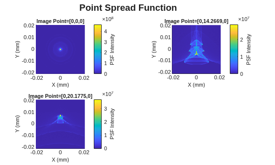
Import an optical system from a shipped ZMX file, and compute the geometric PSF.

opsys = zmximport("DoubleGaussLens.zmx");
psfr = psf(opsys);

Display the PSF image.

h = show(psfr);

Compute Huygens PSF for Multiple Wavelengths

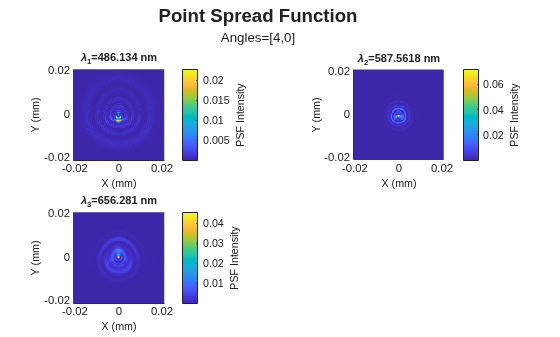
Import an optical system from a shipped ZMX file and compute a wave-optics PSF for the default wavelengths. Center the PSF image on the geometrical image center instead of the chief ray hit position.

opsys = zmximport("DoubleGaussLens.zmx");
fp = fieldPoint(Angles=[4 0]);
psfr = psf(opsys,FieldPoints=fp,Method="Huygens");

Display each wavelength channel in a separate tile.

h = show(psfr);
h.CombineWavelengths = "off";

Compute PSF Metrics

Load the sample Double Gauss lens system using zmximport. Define a field point at an angle of 4 degrees along the x-axis and set the wavelength to 587.56 nm. Compute the geometric PSF for these parameters.

opsys = zmximport("DoubleGaussLens.zmx");
fp = fieldPoint(Angles=[0 4]);
lambda = 587.56;
psfr = psf(opsys, FieldPoints=fp, Wavelengths=lambda, Method="Geometric");

Use the PSF result object, psfr, to extract performance metrics. Calculate the centroid location, the fraction of energy contained within a radius of 0.01 units, and the radius required to capture 80% (0.8) of the total energy.

centroidLocation = centroid(psfr)

centroidLocation = 
centroidLocation(:,:,1) =

  -2.5956e-04


centroidLocation(:,:,2) =

   7.1834e-07

energyAtRadius = encircledEnergyAtRadius(psfr, 0.01)

energyAtRadius = 
0.8635

radius80 = radiusAtEncircledEnergy(psfr, 0.8)

radius80 = 
0.0061

Input Arguments

opsys — Optical system

opticalSystem object

Optical system for which to compute the point spread function, specified as an opticalSystem object.

Name-Value Arguments

Specify optional pairs of arguments as Name1=Value1,...,NameN=ValueN, where Name is the argument name and Value is the corresponding value. Name-value arguments must appear after other arguments, but the order of the pairs does not matter.

Example: psf(opsys,Method="Huygens",OutputResolution=[256 256]) computes a wave-optics PSF image with a width and height of 256 samples.

FieldPoints — Field points for PSF computation

opsys.FieldPoints (default) | FieldAngle object | FieldPosition object | array of FieldAngle or FieldPosition objects

Field points for the PSF computation, specified as a FieldAngle object, a FieldPosition object, or an array of field point objects. Each returned psfr element contains the PSF for one field point.

By default, the FieldPoints value is the FieldPoints property of opsys.

Wavelengths — Wavelengths for PSF computation

opsys.Wavelengths (default) | K-element numeric vector

Wavelengths for PSF computation, specified as an K-element numeric vector. K is the number of wavelengths, and each element of the vector is a wavelength in nanometers. The returned PSF image contains one channel for each specified wavelength.

Data Types: double

Method — PSF computation method

"Geometric" (default) | "Geometric" | "Huygens"

PSF computation method, specified as "Geometric" or "Huygens".

Method	Description
"Geometric"	Trace rays through the optical system and bin ray intersections in the image plane. Use this method for fast analysis when aberrations are large compared to diffraction-limited performance.
"Huygens"	Compute a wave-optics PSF using Huygens propagation. Use this method when diffraction and phase effects are important.

ReferenceWavelengthIndex — Index of reference wavelength

positive integer

Index of the reference wavelength, specified as a positive integer. The reference wavelength is used to determine the chief ray hit position for centering the PSF image.

If you specify Wavelengths and do not specify ReferenceWavelengthIndex, the function uses the index of the median wavelength after sorting the wavelength values. If you do not specify Wavelengths, the reference wavelength is specified by the PrimaryWavelengthIndex property of opsys.

OutputResolution — Resolution of PSF image

[128 128] (default) | 1-by-2 vector of positive integers

Resolution of the PSF image, specified as a 1-by-2 vector of positive integers of the form [width height].

PixelSize — Spatial sampling interval of PSF image

positive scalar

Spatial sampling interval of the PSF image in the image plane, specified as a positive scalar in microns. Use this argument to match the PSF sampling to a sensor pixel pitch or a downstream image simulation. If you do not specify this argument, the function determines the pixel size from the Nyquist sampling rate of the diffraction cutoff frequency of the optical system.

Data Types: double

CenterOnChiefRay — Option to center PSF image on chief ray

true (default) | true or 1 | false or 0

Option to center the PSF image on the chief ray hit position of the reference wavelength, specified as a numeric or logical 1 (true) or 0 (false). If you specify false, the function centers the PSF image on the centroid of the traced ray-spot bounding box across all wavelengths.

Data Types: logical

PupilDensityScale — Scale factor for pupil sampling density

1 (default) | positive scalar

Scale factor for the density of pupil samples used to compute the PSF, specified as a positive scalar. Use larger values to increase the sampling density. Values greater than 2 can significantly increase computation time.

Data Types: double

UseGPU — Option to compute PSF on GPU

"auto" (default) | "auto" | true or 1 | false or 0

Option to compute the PSF on a GPU, specified as "auto", a numeric or logical 1 (true), or a numeric or logical 0 (false). If you specify "auto", the function uses MATLAB GPU option validation to resolve whether to use a GPU. This argument applies to both "Geometric" and "Huygens" methods. GPU computation is especially useful for Huygens PSF because wave-optics computation is more expensive.

Output Arguments

psfr — Point spread function results

array of optics.result.GeometricPSF objects | array of optics.result.HuygensPSF objects

Point spread function results, returned as an array of optics.result.GeometricPSF objects when Method is "Geometric", or an array of optics.result.HuygensPSF objects when Method is "Huygens". The returned array contains one object for each field point specified by FieldPoints.

Each PSF object contains an Image property that stores the PSF intensity as an M-by-N-by-K numeric array. M and N are the output image size, and K is the number of specified wavelengths.

The PSF result objects expose the Image, FieldPoint, Wavelengths, ReferenceWavelength, Position, and CenterOnChiefRay properties.

More About

Point spread function

The point spread function is the image-plane intensity distribution produced by a point source. A PSF can spread over a finite area because of aberrations in the optical system and because of diffraction, even for an ideal optical system.

For a Geometric PSF, pixel values are proportional to the number of traced rays that hit each pixel. Diffraction is not modeled.

For a Huygens PSF, pixel values are wave-optics intensities scaled to the peak intensity of the diffraction-limited system. The peak value of a Huygens PSF corresponds to the Strehl ratio.

Use a Geometric PSF for fast analysis when aberrations dominate the diffraction-limited spot size. Use a Huygens PSF when diffraction effects, phase, or wave-optics metrics such as Strehl ratio are important.

PSF image centering

By default, the psf function centers the PSF image on the chief ray hit position for the reference wavelength. This centering makes centroid offsets useful for measuring wavelength-dependent shifts, chief ray targeting error, and asymmetric aberrations. To center the image on the centroid of the traced ray-spot bounding box across all wavelengths, set CenterOnChiefRay to false.

Algorithms

Pixel Size

If you specify the PixelSize name-value argument, the function uses that value, in microns, as the spatial sampling interval of the output PSF image.

If you do not specify PixelSize, the function determines the pixel size from the Nyquist sampling rate of the diffraction cutoff frequency of the optical system. The function calculates the pixel size as PixelSize = 1/(2*cutoffFrequency), where cutoffFrequency is the diffraction cutoff frequency of the optical system in cycles per micron. For a diffraction-limited system, cutoffFrequency = 1/(wavelength*fNumber), where wavelength is the wavelength in microns and fNumber is the f-number of the optical system.

The specified or automatically determined pixel size and the OutputResolution value together determine the physical extent of the PSF image, which the function stores in the Position property of the returned PSF object.

Sampling

The function uses stratified pupil sampling for Geometric PSF and hexapolar pupil sampling for Huygens PSF. Use PupilDensityScale to control the sampling density.

Version History

Introduced in R2026b