Downlink Shared Channel

The physical downlink shared channel (PDSCH) is used to transmit the downlink shared channel (DL-SCH). The DL-SCH is the transport channel used for transmitting downlink data (a transport block).

DL-SCH Coding

• Transport Block CRC Attachment

• Code Block Segmentation and CRC Attachment

• Channel Coding

• Rate Matching

• Code Block Concatenation

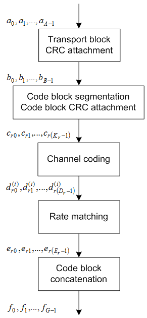
To create the PDSCH payload, a transport block of length A, denoted by $$a_0,a_1,\dots ,a_{A-1}$$, undergoes transport block CRC attachment, code block segmentation and code block CRC attachment, channel coding, rate matching and code block concatenation. The coding steps are illustrated in this block diagram.

Transport Block CRC Attachment

A cyclic redundancy check (CRC) is used for error detection in transport blocks. The entire transport block is used to calculate the CRC parity bits. The transport block is divided by a cyclic generator polynomial, described as $$g_{CRC24A}$$ in section 5.1.1 of [1], to generate 24 parity bits. These parity bits are then appended to the end of the transport block.

Code Block Segmentation and CRC Attachment

The input block of bits to the code segmentation block is denoted by $$b_0,b_1,\dots ,b_{B-1}$$, where $$B=A+24$$. In LTE, a minimum and maximum code block size is specified, so the block sizes are compatible with the block sizes supported by the turbo interleaver.

• The minimum code block size is 40 bits

• The maximum code block size, denoted by Z, is 6144 bits

If the length of the input block, B, is greater than the maximum code block size, the input block is segmented.

When the input block is segmented, it is divided into $$C=\left[B/\left(Z-L\right)\right]$$ smaller blocks, where L is 24. Therefore, $$C=\left[B/6120\right]$$ code blocks.

Each code block has a 24-bit CRC attached to the end, calculated as described in Transport Block CRC Attachment, but the generator polynomial, described as $$g_{CRC24B}$$ in section 5.1.1 of [1] is used.

If required, the algorithm appends filler bits to the start of the segment so that the code block sizes match a set of valid turbo interleaver block sizes. The process is shown in this figure.

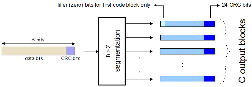
If no segmentation is needed, only one code block is produced. If B is less than the minimum size, filler bits (zeros) are added to the beginning of the code block to achieve a total of 40 bits.

Channel Coding

The code blocks undergo turbo coding. Turbo coding is a form of forward error correction that improves the channel capacity by adding redundant information. The turbo encoder scheme used is a Parallel Concatenated Convolutional Code (PCCC) with two recursive convolutional coders and a “contention-free” Quadratic Permutation Polynomial (QPP) interleaver, as shown in this figure.

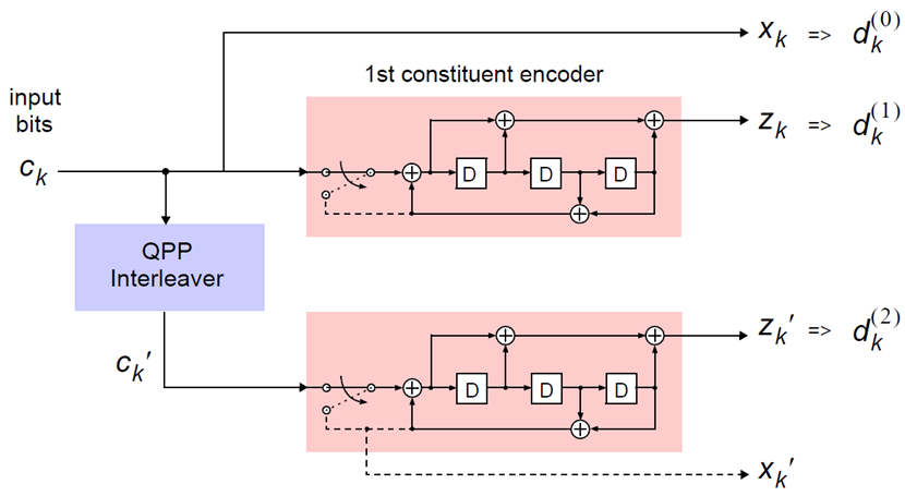
The output of the encoder is three streams, $$d_k^{(0)}$$, $$d_k^{(1)}$$, and $$d_k^{(2)}$$, to achieve a code rate of 1/3.

Constituent Encoders.  The input to the first constituent encoder is the input bit stream to the turbo coding block. The input to the second constituent encoder is the output of the QPP interleaver, a permutation of the input sequence.

Each encoder outputs two sequences, called the systematic sequence and the parity sequence. The systematic sequences are denoted by $$(x_k,{x^{\prime }}_k)$$ and the parity sequences are denoted by $$(z_k,{z^{\prime }}_k)$$. Only one of the systematic sequences ($$x_k$$) is used as an output because the other ($${x^{\prime }}_k$$) is simply a permutation of the chosen systematic sequence. The transfer function for each constituent encoder is given by the following equation.

$$G(D)=\left[1,\frac{g_1(D)}{g_0(D)}\right]$$

The first element, 1, represents the systematic output transfer function. The second element, $$\left(\frac{g_1(D)}{g_0(D)}\right)$$, represents the recursive convolutional output transfer function.

$$g_0(D)=1+D^2+D^3$$

$$g_1(D)=1+D+D^3$$

The output for each sequence can be calculated using the transfer function.

The encoder is initialized with all zeros. If the code block to be encoded is the 0-th and filler bits (F) are used, the input to the encoder ($$c_k$$) is set to zero and the output ($$x_k$$) and ($$z_k$$) set to <NULL> for $$k=0,\dots ,F-1$$.

Trellis Termination for Turbo Encoder.  In a normal convolutional coder, the coder is driven to an all zeros state upon termination by appending zeros to the end of the input data stream. Since the decoder knows the start and end state of the encoder, it can decode the data. Driving a recursive coder to an all zeros state using this method is not possible. To overcome this problem, trellis termination is used.

Upon termination, the tail bits are fed back to the input of each encoder using a switch. The first three tail bits are used to terminate each encoder.

The QPP Interleaver.  The role of the interleaver is to spread the information bits such that in the event of a burst error, the two code streams are affected differently, allowing data to still be recovered.

The output of the interleaver is a permutation of the input data, as shown in these equations.

$${c^{\prime }}_i=c_{\Pi (i)},i=0,1,\dots ,(K-1)$$

$$\Pi (i)=\left(f_{1}i+f_2{i}^2\right)\mathrm{mod}K$$

The variable K is the input length. The variables f₁ and f₂ are coefficients chosen depending on K, in table 5.1.3-3 of [1]. For example, K=40, f₁=3, and f₂=10, yields the following sequence.

$$\Pi (i)=0,13,6,19,12,25,18,31,24,37,30,3,36,9,2,15,8,21,14,27,20,33,26,39,32,5,38,\dots$$

Rate Matching

The rate matching block creates an output bitstream with a desired code rate. Since the number of bits available for transmission depends on the available resources, the rate matching algorithm is capable of producing any rate. The three bitstreams from the turbo encoder are interleaved, followed by bit collection, to create a circular buffer. Bits are selected and pruned from the buffer to create an output bitstream with the desired code rate. The process is illustrated in this figure.

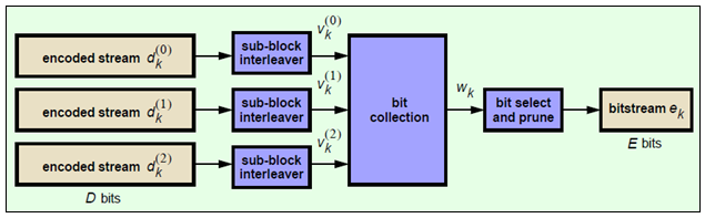
Sub-block Interleaver.  The three sub-block interleavers used in the rate matching block are identical. An interleaver permutes the bits it receives. This makes burst errors easier to correct by preventing consecutive corrupt bits.

The sub-block interleaver reshapes the encoded bit sequence, row-by-row, to form a matrix with $$C_{Subblock}^{TC}=32$$ columns and $$R_{Subblock}^{TC}$$ rows. The variable $$R_{Subblock}^{TC}$$ is determined by finding the minimum integer such that the number of encoded input bits is $$D\le \left(R_{Subblock}^{TC}\times C_{Subblock}^{TC}\right)$$. If $$\left(R_{Subblock}^{TC}\times C_{Subblock}^{TC}\right)>D$$, N_D <NULL>’s are appended to the front of the encoded sequence. In this case, $$N_D+D=\left(R_{Subblock}^{TC}\times C_{Subblock}^{TC}\right)$$.

For blocks $$d_k^{(0)}$$ and $$d_k^{(1)}$$, inter-column permutation is performed on the matrix to reorder the columns as shown in this pattern.

0, 16, 8, 24, 4, 20, 12, 28, 2, 18, 10, 26, 6, 22, 14, 30, 1, 17, 9, 25, 5, 21, 13, 29, 3, 19, 11, 27, 7, 23, 15, 31

The output of the block interleaver for blocks $$d_k^{(0)}$$ and $$d_k^{(1)}$$ is the bit sequence read out column-by-column from the inter-column permuted matrix to create a stream $$K_{\pi }=\left(R_{Subblock}^{TC}\times C_{Subblock}^{TC}\right)$$ bits long.

For block $$d_k^{(2)}$$, the elements of the matrix are permuted separately based on the permutation pattern shown above, but modified to create a permutation which is a function of the variables $$R_{Subblock}^{TC}$$, $$C_{Subblock}^{TC}$$, k, and $$K_{\pi }$$. This process creates three interleaved bitstreams.

$$d_k^{(0)}\to v_k^{(0)}$$

$$d_k^{(1)}\to v_k^{(1)}$$

$$d_k^{(2)}\to v_k^{(2)}$$

Bit Collection, Selection, and Transmission.  The bit collection stage creates a virtual circular buffer by combining the three interleaved encoded bit streams.

The sequences $$v_k^{(1)}$$ and $$v_k^{(2)}$$ are combined by interlacing successive values from each sequence. This combination is then appended to the end of $$v_k^{(0)}$$ to create the circular buffer $$w_k$$ shown in this figure.

Interlacing allows equal levels of protection for each parity sequence.

The algorithm then selects and prunes bits from the circular buffer to create an output sequence length that meets the desired code rate.

The Hybrid Automatic Repeat Request (HARQ) error correction scheme is incorporated into the rate-matching algorithm of LTE. For any desired code rate the coded bits are output serially from the circular buffer from a starting location, given by the redundancy version (RV), wrapping around to the beginning of the buffer if the end of the buffer is reached. NULL bits are discarded. Different RVs, and hence starting points, allow for the retransmission of selected data. The ability to select different starting points enables the following two main methods of recombining data at the receiver in the HARQ process.

• Chase combining — retransmissions contain the same data and parity bit.

• Incremental redundancy — retransmissions contain different information, so the receiver gains knowledge on each retransmission.

Code Block Concatenation

At this stage, the rate-matched code blocks are combined again. This is done by sequentially concatenating the blocks to create the output of the channel coding, $$f_k$$ for $$k=0,\dots ,G-1$$.

PDSCH Processing

• PDSCH Scrambling

• Modulation

• Layer Mapping

• Precoding

• Valid Codeword, Layer and Precoding Scheme Combinations

• Mapping to Resource Elements

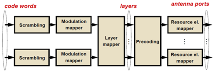
One or two coded transport blocks (codewords) can be transmitted simultaneously on the PDSCH, depending on the precoding scheme used. The DL-SCH codewords undergo scrambling, modulation, layer mapping, precoding and resource element mapping as shown in this figure.

PDSCH Scrambling

The codewords are bit-wise multiplied with an orthogonal sequence and a UE-specific scrambling sequence to create the following sequence of symbols for each codeword, q.

$${\tilde{b}}^{(q)}(0),\dots ,{\tilde{b}}^{(q)}\left(M_{bit}^{(q)}-1\right)$$

The variable $$M_{bit}^{(q)}$$ is the number of bits in codeword q.

The scrambling sequence is pseudo-random, created using a length-31 Gold sequence generator and initialized at the start of each subframe using four parameters:

• the slot number within the radio network temporary identifier associated with the PDSCH transmission, $$n_{RNTI}$$

• the cell ID, $$N_{ID}^{cell}$$

• the slot number within the radio frame, $$n_s$$

• the codeword index, $$q=\left\{0,1\right\}$$.

The initial scrambler state is given by this equation.

$$c_{init}=n_{RNTI}\times 2^{14}+q\times 2^{13}+\lfloor \frac{n_s}{2}\rfloor \times 2^9+N_{ID}^{cell}$$

Scrambling with a cell-specific sequence serves the purpose of intercell interference rejection. When a UE descrambles a received bitstream with a known cell-specific scrambling sequence, interference from other cells will be descrambled incorrectly and therefore only appear as uncorrelated noise.

Modulation

The scrambled codewords undergo QPSK, 16-QAM, 64-QAM, or 256-QAM modulation. This choice creates flexibility to allow the scheme to maximize the data transmitted depending on the channel conditions.

Layer Mapping

The complex symbols are mapped to one, two, or four layers depending on the number of transmit antennas used. The complex modulated input symbols, d(i), are mapped onto v layers, $$x^{(0)}(i),x^{(1)}(i),\dots ,x^{(v-1)}(i)$$.

If a single antenna port is used, only one layer is used. Therefore, $$x^{(0)}(i)=d^{(0)}(i)$$.

Layer Mapping for Transmit Diversity.  If transmitter diversity is used, the input symbols are mapped to layers based on the number of layers.

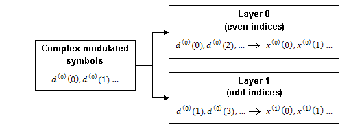
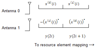
• Two Layers — Even symbols are mapped to layer 0 and odd symbols are mapped to layer 1, as shown in this figure.

  

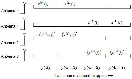
• Four Layers — The input symbols are mapped to layers sequentially, as shown in this figure.

  

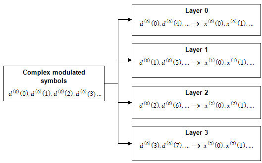
  If the total number of input symbols is not an integer multiple of four, two null symbols are appended to the end. Since the original number of symbols is always an integer multiple of two, the new total is an integer multiple of four.

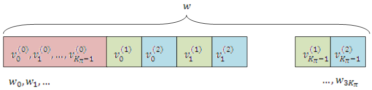
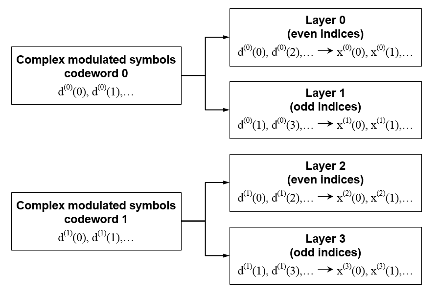
Layer Mapping for Spatial Multiplexing.  In the case of spatial multiplexing, the number of layers used is always less than or equal to the number of antenna ports used for transmission of the physical channel.

 One Layer

If one layer is used, $$x^{(0)}(i)=d^{(0)}(i)$$.

 Two Layers

• One Codeword — Even symbols are mapped to layer 0 and odd symbols are mapped to layer 1, as shown in the following figure.

  

• Two Codewords — Codeword 0 is mapped to layer 0 and codeword 1 is mapped to layer 1, as shown in the following figure.

  

 Three Layers

In the case of three layers, codeword 0 is mapped to layer 0 and even symbols within codeword 1 are mapped to layer 1 and odd symbols within codeword 1 are mapped to layer 2.

 Four Layers

In the case of four layers, two codewords must be used. In this case, the even symbols of codeword 0 are mapped to layer 0, and the odd symbols are mapped to layer 1. The even symbols of codeword 1 are mapped to layer 2, and the odd symbols are mapped to layer 3.

Precoding

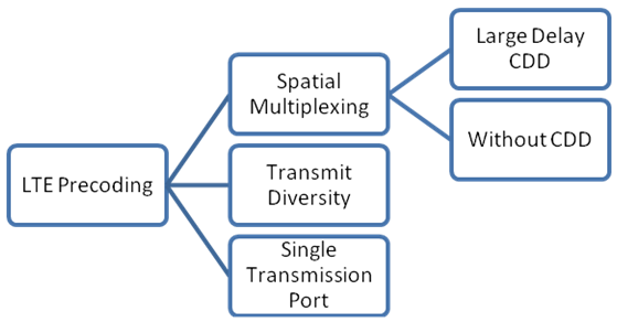
Three types of precoding are available in LTE for the PDSCH: spatial multiplexing, transmit diversity, and single antenna port transmission. Within spatial multiplexing, there are two schemes: precoding with large delay cyclic delay diversity (CDD), also known as open loop spatial multiplexing, and precoding without CDD, also known as closed loop spatial multiplexing. The various types of precoding are illustrated in this tree diagram.

The precoder takes a block from the layer mapper, $$x^{(0)}(i),x^{(1)}(i),\dots ,x^{(v-1)}(i)$$, and generates a sequence for each antenna port, $$y^{(p)}(i)$$. The variable p is the transmit antenna port number, and can assume values of {0}, {0,1}, or {0,1,2,3}.

Single Antenna Port Precoding.  For transmission over a single antenna port, no processing is carried out, as shown in this equation.

$$y^{(p)}(i)=x^{(0)}(i)$$

Precoding for Large Delay CDD Spatial Multiplexing.  CDD operation applies a cyclic shift, which is a delay of $$N_{FFT}/v$$ samples to each antenna, where $$N_{FFT}$$ is the size of the OFDM FFT. The use of CDD improves the robustness of performance by randomizing the channel frequency response, reducing the probability of deep fading.

Precoding with CDD for spatial multiplexing is defined by the following equation.

$$\left(\begin{array}{c}{y}^{(0)}(i)\\ ⋮\\ y^{(p-1)}(i)\end{array}\right)=W(i)\times D(i)\times U\times \left(\begin{array}{c}{x}^{(0)}(i)\\ ⋮\\ x^{(v-1)}(i)\end{array}\right)$$

Values of the precoding matrix, $$W(i)$$, of size $$P\times v$$, are selected from a codebook configured by the eNodeB and user equipment. The precoding codebook is described in Spatial Multiplexing Precoding Codebook. Every group of symbols at index i across all available layers can use a different precoding matrix, if required. The supporting matrices, $$D(i)$$and U, are given for various numbers of layers in the following table.

Number of layers, $$\upsilon$$	U	$$D(i)$$
2	$$\frac{1}{\sqrt{2}}\left(\begin{array}{cc}1& 1\\ 1& e^{-j2\pi /2}\end{array}\right)$$	$$\left(\begin{array}{cc}1& 0\\ 0& e^{-j2\pi i/2}\end{array}\right)$$
3	$$\frac{1}{\sqrt{3}}\left(\begin{array}{ccc}1& 1& 1\\ 1& e^{-j2\pi /3}& e^{-j4\pi /3}\\ 1& e^{-j4\pi /3}& e^{-j8\pi /3}\end{array}\right)$$	$$\left(\begin{array}{ccc}1& 0& 0\\ 0& e^{-j2\pi i/3}& 0\\ 0& 0& e^{-j4\pi i/3}\end{array}\right)$$
4	$$\frac{1}{2}\left(\begin{array}{cccc}1& 1& 1& 1\\ 1& e^{-j2\pi /4}& e^{-j4\pi /4}& e^{-j6\pi /4}\\ 1& e^{-j4\pi /4}& e^{-j8\pi /4}& e^{-j12\pi /4}\\ 1& e^{-j6\pi /4}& e^{-j12\pi /4}& e^{-j18\pi /4}\end{array}\right)$$	$$\left(\begin{array}{cccc}1& 0& 0& 0\\ 0& e^{-j2\pi i/4}& 0& 0\\ 0& 0& e^{-j4\pi i/4}& 0\\ 0& 0& 0& e^{-j6\pi i/4}\end{array}\right)$$

Precoding for Spatial Multiplexing without CDD.  Precoding for spatial multiplexing without CDD is defined by the following equation.

$$\left(\begin{array}{c}{y}^{(0)}(i)\\ ⋮\\ y^{(p-1)}(i)\end{array}\right)=W(i)\times \left(\begin{array}{c}{x}^{(0)}(i)\\ ⋮\\ x^{(v-1)}(i)\end{array}\right)$$

Values of the precoding matrix, $$W(i)$$, of size $$P\times v$$, are selected from a codebook configured by the eNodeB and user equipment. Every group of symbols at index i across all available layers can use a different precoding matrix if required. For more information on the precoding codebook, see Spatial Multiplexing Precoding Codebook.

Spatial Multiplexing Precoding Codebook.  The precoding matrices for antenna ports {0,1} are given in the following table.

Codebook index	Number of layers, $$\upsilon$$
	1	2
0	$$\frac{1}{\sqrt{2}}\left(\begin{array}{c}1\\ 1\end{array}\right)$$	$$\frac{1}{\sqrt{2}}\left(\begin{array}{cc}1& 0\\ 0& 1\end{array}\right)$$
1	$$\frac{1}{\sqrt{2}}\left(\begin{array}{c}1\\ -1\end{array}\right)$$	$$\frac{1}{2}\left(\begin{array}{cc}1& 1\\ 1& -1\end{array}\right)$$
2	$$\frac{1}{\sqrt{2}}\left(\begin{array}{c}1\\ j\end{array}\right)$$	$$\frac{1}{2}\left(\begin{array}{cc}1& 1\\ j& -j\end{array}\right)$$
3	$$\frac{1}{\sqrt{2}}\left(\begin{array}{c}1\\ -j\end{array}\right)$$	—

The precoding matrices for antenna ports {0,1,2,3} are given in the following table.

Codebook index	un	Number of layers, v
		1	2	3	4
0	$$u_0=[{\begin{array}{cccc}1& -1& -1& -1]\end{array}}^T$$	$$W_0^{\left\{1\right\}}$$	$$\frac{W_0^{\left\{14\right\}}}{\sqrt{2}}$$	$$\frac{W_0^{\left\{124\right\}}}{\sqrt{3}}$$	$$\frac{W_0^{\left\{1234\right\}}}{2}$$
1	$$u_1=[{\begin{array}{cccc}1& -j& 1& j]\end{array}}^T$$	$$W_1^{\left\{1\right\}}$$	$$\frac{W_1^{\left\{12\right\}}}{\sqrt{2}}$$	$$\frac{W_1^{\left\{123\right\}}}{\sqrt{3}}$$	$$\frac{W_1^{\left\{1234\right\}}}{2}$$
2	$$u_2=[{\begin{array}{cccc}1& 1& -1& 1]\end{array}}^T$$	$$W_2^{\left\{1\right\}}$$	$$\frac{W_2^{\left\{12\right\}}}{\sqrt{2}}$$	$$\frac{W_2^{\left\{123\right\}}}{\sqrt{3}}$$	$$\frac{W_2^{\left\{3214\right\}}}{2}$$
3	$$u_3=[{\begin{array}{cccc}1& j& 1& -j]\end{array}}^T$$	$$W_3^{\left\{1\right\}}$$	$$\frac{W_3^{\left\{12\right\}}}{\sqrt{2}}$$	$$\frac{W_3^{\left\{123\right\}}}{\sqrt{3}}$$	$$\frac{W_3^{\left\{3214\right\}}}{2}$$
4	$$u_4={\left[\begin{array}{cccc}1& \frac{-1-j}{\sqrt{2}}& -j& \frac{1-j}{\sqrt{2}}\end{array}\right]}^T$$	$$W_4^{\left\{1\right\}}$$	$$\frac{W_4^{\left\{14\right\}}}{\sqrt{2}}$$	$$\frac{W_4^{\left\{124\right\}}}{\sqrt{3}}$$	$$\frac{W_4^{\left\{1234\right\}}}{2}$$
5	$$u_5={\left[\begin{array}{cccc}1& \frac{1-j}{\sqrt{2}}& j& \frac{-1-j}{\sqrt{2}}\end{array}\right]}^T$$	$$W_5^{\left\{1\right\}}$$	$$\frac{W_5^{\left\{14\right\}}}{\sqrt{2}}$$	$$\frac{W_5^{\left\{124\right\}}}{\sqrt{3}}$$	$$\frac{W_5^{\left\{1234\right\}}}{2}$$
6	$$u_6={\left[\begin{array}{cccc}1& \frac{1+j}{\sqrt{2}}& -j& \frac{-1+j}{\sqrt{2}}\end{array}\right]}^T$$	$$W_6^{\left\{1\right\}}$$	$$\frac{W_6^{\left\{13\right\}}}{\sqrt{2}}$$	$$\frac{W_6^{\left\{134\right\}}}{\sqrt{3}}$$	$$\frac{W_6^{\left\{1324\right\}}}{2}$$
7	$$u_7={\left[\begin{array}{cccc}1& \frac{-1+j}{\sqrt{2}}& j& \frac{1+j}{\sqrt{2}}\end{array}\right]}^T$$	$$W_7^{\left\{1\right\}}$$	$$\frac{W_7^{\left\{13\right\}}}{\sqrt{2}}$$	$$\frac{W_7^{\left\{134\right\}}}{\sqrt{3}}$$	$$\frac{W_7^{\left\{1324\right\}}}{2}$$
8	$$u_8={[\begin{array}{cccc}1& -1& 1& 1\end{array}]}^T$$	$$W_8^{\left\{1\right\}}$$	$$\frac{W_8^{\left\{12\right\}}}{\sqrt{2}}$$	$$\frac{W_8^{\left\{124\right\}}}{\sqrt{3}}$$	$$\frac{W_8^{\left\{1234\right\}}}{2}$$
9	$$u_9=[{\begin{array}{cccc}1& -j& -1& -j]\end{array}}^T$$	$$W_9^{\left\{1\right\}}$$	$$\frac{W_9^{\left\{14\right\}}}{\sqrt{2}}$$	$$\frac{W_9^{\left\{134\right\}}}{\sqrt{3}}$$	$$\frac{W_9^{\left\{1234\right\}}}{2}$$
10	$$u_{10}=[{\begin{array}{cccc}1& 1& 1& -1]\end{array}}^T$$	$$W_{10}^{\left\{1\right\}}$$	$$\frac{W_{10}^{\begin{array}{l}\{13\\ \}\end{array}}}{\sqrt{2}}$$	$$\frac{W_{10}^{\left\{123\right\}}}{\sqrt{3}}$$	$$\frac{W_{10}^{\left\{1324\right\}}}{2}$$
11	$$u_{11}=[{\begin{array}{cccc}1& j& -1& j]\end{array}}^T$$	$$W_{11}^{\left\{1\right\}}$$	$$\frac{W_{11}^{\left\{13\right\}}}{\sqrt{2}}$$	$$\frac{W_{11}^{\left\{134\right\}}}{\sqrt{3}}$$	$$\frac{W_{11}^{\left\{1324\right\}}}{2}$$
12	$$u_{12}=[{\begin{array}{cccc}1& -1& -1& 1]\end{array}}^T$$	$$W_{12}^{\left\{1\right\}}$$	$$\frac{W_{12}^{\left\{12\right\}}}{\sqrt{2}}$$	$$\frac{W_{12}^{\left\{123\right\}}}{\sqrt{3}}$$	$$\frac{W_{12}^{\left\{1324\right\}}}{2}$$
13	$$u_{13}=[{\begin{array}{cccc}1& -1& 1& -1]\end{array}}^T$$	$$W_{13}^{\left\{1\right\}}$$	$$\frac{W_{13}^{\left\{13\right\}}}{\sqrt{2}}$$	$$\frac{W_{13}^{\left\{123\right\}}}{\sqrt{3}}$$	$$\frac{W_{13}^{\left\{1324\right\}}}{2}$$
14	$$u_{14}=[{\begin{array}{cccc}1& 1& -1& -1]\end{array}}^T$$	$$W_{14}^{\left\{1\right\}}$$	$$\frac{W_{14}^{\left\{13\right\}}}{\sqrt{2}}$$	$$\frac{W_{14}^{\left\{123\right\}}}{\sqrt{3}}$$	$$\frac{W_{14}^{\left\{3214\right\}}}{2}$$
15	$$u_{15}=[{\begin{array}{cccc}1& 1& 1& 1]\end{array}}^T$$	$$W_{15}^{\left\{1\right\}}$$	$$\frac{W_{15}^{\left\{12\right\}}}{\sqrt{2}}$$	$$\frac{W_{15}^{\left\{123\right\}}}{\sqrt{3}}$$	$$\frac{W_{15}^{\left\{1234\right\}}}{2}$$

The precoding matrix, $$W_n^{\left\{s\right\}}$$, is the matrix defined by the columns in set $$\left\{s\right\}$$ by the following equation.

$$W_n=I-2u_n{u}_n^H/u_n^H{u}_n$$

In the preceding equation, I is a 4-by-4 identity matrix. The vector $$u_n$$ is given in the preceding table.

Precoding for Transmit Diversity.  Precoding for transmit diversity is available on two or four antenna ports.

 Two Antenna Ports

An Alamouti scheme is used for precoding, which defines the relationship between input and output as shown in the following equation.

$$\left(\begin{array}{c}{y}^{(0)}(2i)\\ y^{(1)}(2i)\\ y^{(0)}(2i+1)\\ y^{(1)}(2i+1)\end{array}\right)=\frac{1}{\sqrt{2}}\left(\begin{array}{cccc}1& 0& j& 0\\ 0& -1& 0& j\\ 0& 1& 0& j\\ 1& 0& -j& 0\end{array}\right)\left(\begin{array}{c}\mathrm{Re}\left\{x^{(0)}(i)\right\}\\ \mathrm{Re}\left\{x^{(1)}(i)\right\}\\ \mathrm{Im}\left\{x^{(0)}(i)\right\}\\ \mathrm{Im}\left\{x^{(1)}(i)\right\}\end{array}\right)$$

In the Alamouti scheme, two consecutive symbols, $$x^{(0)}(i)$$ and $$x^{(1)}(i)$$, are transmitted in parallel using two antennas with the following mapping, where the asterisk symbol (*) denotes the complex conjugate operation.

Since any two columns in the precoding matrix are orthogonal, the two symbols, $$x^{(0)}(i)$$ and $$x^{(1)}(i)$$, can be separated at the UE.

 Four Antenna Ports

Precoding for the four antenna port case defines the relationship between the input and output as shown in the following equation.

$$\left(\begin{array}{c}{y}^{(0)}(4i)\\ y^{(1)}(4i)\\ y^{(2)}(4i)\\ y^{(3)}(4i)\\ y^{(0)}(4i+1)\\ y^{(1)}(4i+1)\\ y^{(2)}(4i+1)\\ y^{(3)}(4i+1)\\ y^{(0)}(4i+2)\\ y^{(1)}(4i+2)\\ y^{(2)}(4i+2)\\ y^{(3)}(4i+2)\\ y^{(0)}(4i+3)\\ y^{(1)}(4i+3)\\ y^{(2)}(4i+3)\\ y^{(3)}(4i+3)\end{array}\right)=\frac{1}{\sqrt{2}}\left(\begin{array}{cccccccc}1& 0& 0& 0& j& 0& 0& 0\\ 0& 0& 0& 0& 0& 0& 0& 0\\ 0& -1& 0& 0& 0& j& 0& 0\\ 0& 0& 0& 0& 0& 0& 0& 0\\ 0& 1& 0& 0& 0& j& 0& 0\\ 0& 0& 0& 0& 0& 0& 0& 0\\ 1& 0& 0& 0& -j& 0& 0& 0\\ 0& 0& 0& 0& 0& 0& 0& 0\\ 0& 0& 0& 0& 0& 0& 0& 0\\ 0& 0& 1& 0& 0& 0& j& 0\\ 0& 0& 0& 0& 0& 0& 0& 0\\ 0& 0& 0& -1& 0& 0& 0& j\\ 0& 0& 0& 0& 0& 0& 0& 0\\ 0& 0& 0& 1& 0& 0& 0& j\\ 0& 0& 0& 0& 0& 0& 0& 0\\ 0& 0& 1& 0& 0& 0& -j& 0\end{array}\right)\left(\begin{array}{c}\mathrm{Re}\left\{x^{(0)}(i)\right\}\\ \mathrm{Re}\left\{x^{(1)}(i)\right\}\\ \mathrm{Re}\left\{x^{(2)}(i)\right\}\\ \mathrm{Re}\left\{x^{(3)}(i)\right\}\\ \mathrm{Im}\left\{x^{(0)}(i)\right\}\\ \mathrm{Im}\left\{x^{(1)}(i)\right\}\\ \mathrm{Im}\left\{x^{(2)}(i)\right\}\\ \mathrm{Im}\left\{x^{(3)}(i)\right\}\end{array}\right)$$

In this scheme, two consecutive symbols are transmitted in parallel in two symbol periods using four antennas with this mapping, where the asterisk symbol (*) denotes the complex conjugate operation.

Valid Codeword, Layer and Precoding Scheme Combinations

The valid numbers of codewords and layers for each precoding scheme, as described in previous sections, are summarized in these tables.

Single Antenna Port

Codewords	Layers
1	1

Transmit Diversity

Codewords	Layers
1	2
1	4

Spatial Multiplexing

Codewords	Layers
1	1
1	2
2	2
2	3
2	4

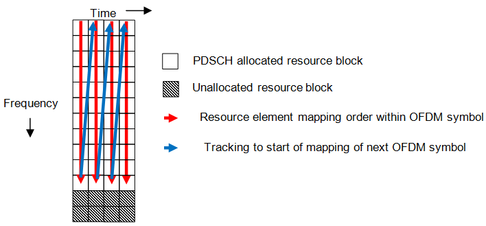
Mapping to Resource Elements

For each of the antenna ports used for transmission of the PDSCH, the block of complex valued symbols, $$y^{(p)}(i)$$, are mapped in sequence to resource elements not occupied by the PCFICH, PHICH, PDCCH, PBCH, or synchronization and reference signals. The number of resource elements mapped to is controlled by the number of resource blocks allocated to the PDSCH. The symbols are mapped by increasing the subcarrier index and mapping all available REs within allocated resource blocks for each OFDM symbol as shown in this figure.

References

[1] 3GPP TS 36.212. “Evolved Universal Terrestrial Radio Access (E-UTRA); Multiplexing and channel coding.” 3rd Generation Partnership Project; Technical Specification Group Radio Access Network. URL: https://www.3gpp.org.